Upgrade to Pro — share decks privately, control downloads, hide ads and more …

Controllability of Keplerian Motion with Low-Thrust Control Systems

GdR MOA 2015
December 03, 2015

Controllability of Keplerian Motion with Low-Thrust Control Systems

by Z. Chen

GdR MOA 2015

December 03, 2015
Tweet

More Decks by GdR MOA 2015

Other Decks in Science

Transcript

  1. Outline Definitions and notations Orbital transfer problem Orbital insertion problem

    De-orbital problem Controllability of Keplerian Motion with Low-Thrust Control Systems Zheng Chen1 and Yacine Chitour1,2 1. University Paris-Sud & CNRS, France 2. L2S, CentraleSup´ elec, France Journ´ ees annuelles 2015 du GdR MOA, December 2–4, 2015
  2. Outline Definitions and notations Orbital transfer problem Orbital insertion problem

    De-orbital problem Outline 1 Definitions and notations Dynamics of Two-Body Problem Properties of drift vector field 2 Orbital transfer problem Controllability for linearised system Controllability for OTPs 3 Orbital insertion problem Controllability for OIPs Numerical method for OIPs 4 De-orbital problem
  3. Outline Definitions and notations Orbital transfer problem Orbital insertion problem

    De-orbital problem Dynamics of Two-Body Problem On the interval [0, t f ], the dynamics of a satellite moving around the Earth is ⌃sat : 8 > < > : ˙ r (t) = v (t), ˙ v (t) = µ k r ( t )k3 r (t) + ⌧( t ) m ( t ) , ˙ m(t) = k ⌧(t) k, where m 2 R⇤ + , r 2 R3\{0}, v 2 R3, µ > 0, > 0, and the control (or thrust) vector ⌧ 2 R3 takes values in the admissible set T (⌧ max ) = n⌧ 2 R3 | k⌧k  ⌧ max o, where ⌧ max > 0 is a constant. Geocentric Inertial Cartesian Coordinate System.
  4. Outline Definitions and notations Orbital transfer problem Orbital insertion problem

    De-orbital problem Constant mass dynamics Let X = R3\{0} ⇥ R3 and x = ( r , v ), we define the two vector fields f 0, f 1 on X by f 0 : X ! R6, f 0 ( x ) = ✓ v µ k r k3 r ◆ , f 1 : X ! R6⇥3, f 1 ( x ) = ✓ 0 I3 ◆ . For every " > 0, we consider the control-a ne system ⌃" given by ⌃" : ˙ x (t) = f 0 ( x (t)) + f 1 ( x (t)) u (t), where the control u 2 R3 takes values in B" = { u 2 R3 | k u k  "}. For every point x 2 X and every u 2 B" , we define by f : X ⇥ B" ! T x X, ( x , u ) 7! f ( x , u ) = f 0 ( x ) + f 1 ( x ) u , where f 0 and f 1 are referred to as the drift vector field and the control vector field, respectively.
  5. Outline Definitions and notations Orbital transfer problem Orbital insertion problem

    De-orbital problem Main properties of the drift vector field f 0 For every x 2 X, we use x to denote the restriction to R+ of the maximum trajectory of f 0 starting at x , i.e., x is defined on some interval [0, t f ( x )) where t f ( x )  1. Property (First integrals) For every x 2 X, if x (t) = (˜ r (t), ˜ v (t)) on [0, t f ( x )), the quantities h = ˜ r (t) ⇥ ˜ v (t), L = ˜ v (t) ⇥ h µ ˜ r (t) k ˜ r (t) k , E = k ˜ v (t) k2 2 µ k ˜ r (t) k , are constant along x , and the corresponding constant values are the angular momentum vector h 2 R3, the Laplace vector L 2 R3 and the mechanical energy of a unit mass E 2 R.
  6. Outline Definitions and notations Orbital transfer problem Orbital insertion problem

    De-orbital problem Main properties of the drift vector field f 0 Property (Straight line) Let x 2 X with h = 0, i.e., ˜ r and ˜ v are collinear. Then the trajectory x is a straight line. Property (Conic section) Let x 2 X with h 6= 0, i.e., ˜ r and ˜ v are not collinear. Then, the locus of x defines a conic section lying in a two-dimensional plane perpendicular to h , called the orbital plane. Let k L kk˜ r k cos(✓) = LT · ˜ r , one gets h 6= 0 !k ˜ r (t) k= h 2 µ[1+ k L k cos(✓(t))/µ] .
  7. Outline Definitions and notations Orbital transfer problem Orbital insertion problem

    De-orbital problem Main properties of the drift vector field f 0 (a : R3\{0} ⇥ R3 ! a( r , v ) = µ 2 E , e : R3\{0} ⇥ R3 ! e( r , v ) =k L k /µ, =)k ˜ r (t) k= a(1 e2) 1 + e cos(✓(t)) . 0  e < 1 =) E < 0. Definition (Periodic region) P = {( r , v ) 2 R3\{0} ⇥ R3 | E < 0, h 6= 0}.
  8. Outline Definitions and notations Orbital transfer problem Orbital insertion problem

    De-orbital problem Main properties of the drift vector field f 0 r p : P ! R, r p ( r , v ) = a( r , v )(1 e( r , v )), r a : P ! R, r a ( r , v ) = a( r , v )(1 + e( r , v )). ‹ ‹ ષ ” ” ˜ ˜ ‡ ‡ Y Z X   Š Š ‹ ‹ Ʌ ɘ Equatorial plane 2a ra rp Orbital plane ߠ r v Apogee Perigee
  9. Outline Definitions and notations Orbital transfer problem Orbital insertion problem

    De-orbital problem Admissible region Definition (Admissible region) We say the set A = ( r , v ) 2 P | k r k> r c > 0 is the admissible region for Keplerian motion or/and controlled Keplerian motion. Definition (Stable region P+ and unstable region P ) P+ = {( r , v ) 2 P | r p ( r , v ) > r c }, P = {( r , v ) 2 P | k r k> r c , r p ( r , v ) < r c < r a ( r , v )}. xi xf xf xi xi xf rc rc rc xi xf xf xi xi xf rc rc rc xi xf xf xi xi xf rc rc rc
  10. Outline Definitions and notations Orbital transfer problem Orbital insertion problem

    De-orbital problem Controlled Problems The problem of controlling a satellite from a point xi = ( ri , vi ) in P+ to a point xf = ( rf , vf ) 6= xi in P+ is the orbital transfer problem (OTP). The problem of controlling a satellite from an initial point xi = ( ri , vi ) 2 P to a final point xf = ( rf , vf ) 2 P+ is the orbit insertion problem (OIP). The problem of controlling a satellite from an initial point xi = ( ri , vi ) 2 P+ to a final point xf = ( rf , vf ) 2 P is the de-orbit problem (DOP). xi xf xf xi xi xf rc rc rc xi xf xf xi xi xf rc rc rc xi xf xf xi xi xf rc rc rc
  11. Outline Definitions and notations Orbital transfer problem Orbital insertion problem

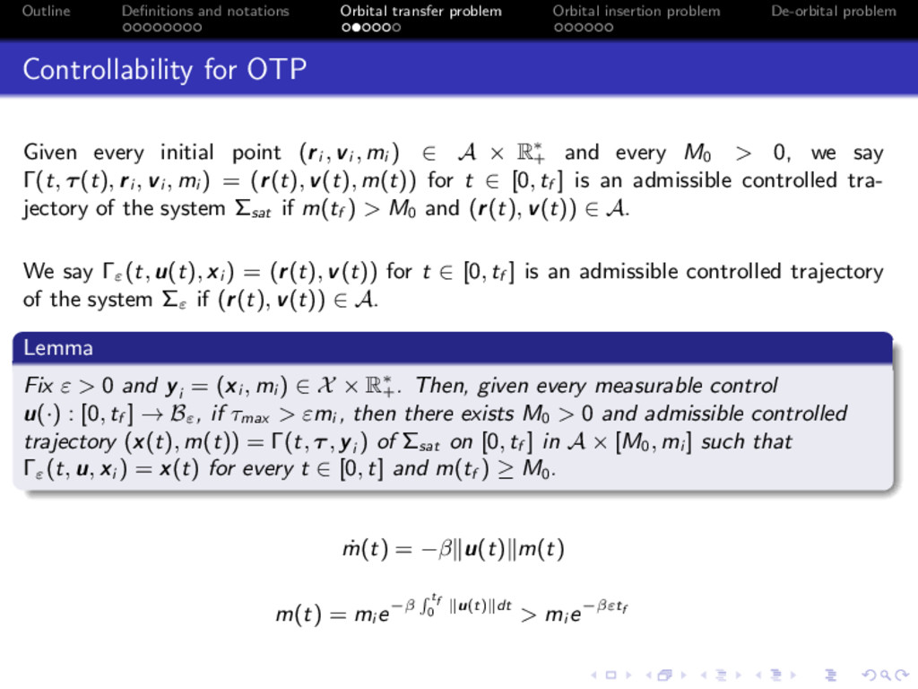
    De-orbital problem Controllability for OTP Given every initial point ( ri , vi , m i ) 2 A ⇥ R⇤ + and every M0 > 0, we say (t, ⌧(t), ri , vi , m i ) = ( r (t), v (t), m(t)) for t 2 [0, t f ] is an admissible controlled tra- jectory of the system ⌃ sat if m(t f ) > M0 and ( r (t), v (t)) 2 A. We say " (t, u (t), xi ) = ( r (t), v (t)) for t 2 [0, t f ] is an admissible controlled trajectory of the system ⌃" if ( r (t), v (t)) 2 A. Lemma Fix " > 0 and yi = ( xi , m i ) 2 X ⇥ R⇤ + . Then, given every measurable control u (·) : [0, t f ] ! B" , if ⌧ max > "m i , then there exists M0 > 0 and admissible controlled trajectory ( x (t), m(t)) = (t, ⌧, yi ) of ⌃ sat on [0, t f ] in A ⇥ [M0, m i ] such that " (t, u , xi ) = x (t) for every t 2 [0, t] and m(t f ) M0 . ˙ m(t) = k u (t)km(t) m(t) = m i e R tf 0 k u ( t )k dt > m i e " tf
  12. Outline Definitions and notations Orbital transfer problem Orbital insertion problem

    De-orbital problem Controllability for OTP Lemma (Connectedness of A) The admissible set A is an arc-connected subset of P, i.e., for every initial point xi 2 A and every final point xf 2 A, there exists a continuous path f : [0, 1] ! A, 7! x ( ) such that x (0) = xi and x (1) = xf . Lemma (Connectedness of P+) The set P+ is a connected subset of A.
  13. Outline Definitions and notations Orbital transfer problem Orbital insertion problem

    De-orbital problem Linearized system ⌃⇤ " ( (t, ¯ u (t), x0 )) Given a control ¯ u (·) : [0, t f ] ! B" , the linearized system ⌃⇤ " ( (t, ¯ u , xi )) along the controlled trajectory ¯ x (t) = " (t, ¯ u , xi ) of ⌃" is defined as ⌃⇤ " ( (t, ¯ u , xi )) : ˙ (t) = A(t) (t) + B(t) u (t), where (t) = ( r (t), v (t)) 2 R6, A(t) = f x (¯ x (t), ¯ u (t)), and B(t) = f u (¯ x (t), ¯ u (t)) on [0, t f ].
  14. Outline Definitions and notations Orbital transfer problem Orbital insertion problem

    De-orbital problem Controllability for OTP Lemma (Local Controllability, Eduardo D. Sontag, 1998) The linearized system ⌃⇤ " ( (t, ¯ u (t), x0 )) along a curve (t, ¯ u (t), x0 ) on [0, t f ] is controllable if rank ([B0 (⌧), B1 (⌧), · · · , B k (⌧)]) = n for a time ⌧ 2 [t0, t f ], where B i +1 (t) = A(t)B i (t) dBi ( t ) dt . A = f x = " 0 I3 µ k r k3 3 + 3 µ k r k5 rrT 0 # B = f u =  0 I3 [B0 (t), B1 (t)] =  0 I3 I3 0 ! X0 ! Xf ! Y! Z!
  15. Outline Definitions and notations Orbital transfer problem Orbital insertion problem

    De-orbital problem Controllability for OTP xf x0 Ȟ(t , 0 , x0 ) Ȟ(t , u(t) , x0 ) Ȟ(t , 0 , x1 ) Ȟ(t , u(t) , x1 ) xf x0 xf x0 Ȟ(t , 0 , x1 ) Ȟ(t , u(t) , x1 ) x1 x2 For every µ > 0 and > 0, the system ⌃" is controllable in P+ if ⌧ max > 0.
  16. Outline Definitions and notations Orbital transfer problem Orbital insertion problem

    De-orbital problem Controllability for OIPs Assume that, for every point ( xi , m i ) 2 P ⇥ R⇤ + , there exists ⌧ max > 0, a finite time t f > 0 ,and a control ˜ ⌧(·) : [0, t f ] ! T (⌧ max ) such that along the controlled trajectory (˜ x , ˜ m) = (t, ˜ ⌧(t), xi , m i ) on [0, t f ], we have ˜ x (t) 2 A on [0, t f ], ˜ m(t f ) > 0, and r p (˜ x (t f )) > r c . Then, the system ⌃ sat is controllable for OIP from ( xi , m i ). xi xf xf xi xi xf rc rc rc xi xf xf xi xi xf rc rc rc xi xf xf xi xi xf rc rc rc
  17. Outline Definitions and notations Orbital transfer problem Orbital insertion problem

    De-orbital problem Numerical method for OIPs Lemma For every > 0, µ > 0, and point yi = ( xi , m i ) in P ⇥ R⇤ + , there exists ˜ ⌧ max > 0 such that the following holds: 1) if ⌧ max > ˜ ⌧ max , there exists a control ⌧(·) taking values in T (⌧ max ) and a finite time t f > 0 such that, along the controlled trajectory ( x (t), m(t)) = (t, ⌧, yi , m i ) on [0, t f ], we have x (t) 2 A on [0, t f ], m(t f ) > 0, and r p ( x (t f )) > r c ; 2) if ⌧ max  ˜ ⌧ max , for every control ⌧(·) taking values in T (⌧ max ), the controlled trajectory ( x (·), m(·)) = (·, ⌧, yi , m i ) does not reach P+ ⇥ R⇤ + . An OIP is controllable if ⌧ max is bigger than a specific value ˜ ⌧ max > 0.
  18. Outline Definitions and notations Orbital transfer problem Orbital insertion problem

    De-orbital problem Numerical method for OIPs Definition (Optimal control problem (OCP) for OIP) Given every initial point ( xi , m i ) 2 P ⇥ R⇤ + and ⌧ max > 0, the optimal control problem for OIP consists of steering a satellite by ⌧(·) 2 T (⌧ max ) on a time interval [0, t f ] such that, along the controlled trajectory ( r (t), v (t), m(t)) = (t, ⌧(t), xi , m i ), the time t f is the first occurence for k r (t f )k = r p ( r (t f ), v (t f )), i.e., k r (t)k > r p ( r (t), v (t)) on [0, t f ), and r p ( r (t f ), v (t f )) is maximized, i.e., the cost functional is J = Z tf 0 d dt r p ( r (t), v (t))dt. Let ˜ t f > 0 be the optimal final time of the OCP for OIP, and let (˜ x (·), ˜ m(·)) on [0, ˜ t f ] be the optimal controlled trajectory associated with the optimal control ˜ ⌧ 2 T (⌧ max ). According to the Pontryagin Maximum Principle, we define a function s : R+ ! R, s(⌧) = r p (˜ x (˜ t f )) r c . s is a function of ⌧ max and a simple bisection method can solve ˜ ⌧ max such that s(˜ ⌧ max ) = 0.
  19. Outline Definitions and notations Orbital transfer problem Orbital insertion problem

    De-orbital problem Numerical method for OIPs I sp = 2000 s =) = 5.102 ⇥ 10 5 m 2, m i = 150 kg. k ri k = r e + 110, 000 m, k vi k = 7, 879.5 m/s, ⌘ i = 5 . k r1k = r e + 379, 494 m, k v1k = 7, 562.0 m/s, ⌘1 = 4.3517 . k r2k = r e + 599, 351 m, k v2k = 7, 312.0 m/s, ⌘2 = 3.0132 .
  20. Outline Definitions and notations Orbital transfer problem Orbital insertion problem

    De-orbital problem Numerical method for OIPs 0 500 1000 1500 2000 2500 3000 3500 4000 4500 5.8 6 6.2 6.4 6.6 6.8 7 7.2 x 10⁶ Time (s) r c r r p r i r 1 r 2 r pi r p1 r p2
  21. Outline Definitions and notations Orbital transfer problem Orbital insertion problem

    De-orbital problem Numerical method for OIPs −8 −6 −4 −2 0 2 4 6 8 x 10⁶ −6 −4 −2 0 2 4 6 8 x 10⁶ X (m) Y (m) r c x i Controlled trajectory Periodic trajectory Surface of atmosphere
  22. Outline Definitions and notations Orbital transfer problem Orbital insertion problem

    De-orbital problem Controllability for DOP Let us define a system ˜ ⌃ sat associated with ⌃ sat as ˜ ⌃ sat : 8 > < > : ˙ r (t) = v (t), ˙ v (t) = µ k r ( t )k3 r (t) + ⌧( t ) m ( t ) , ˙ m(t) = + k⌧(t)k. We define ˜(t, ⌧(t), yi ) the corresponding trajectory of ˜ ⌃ sat for some positive times. Remark For every controlled trajectory ( r (t), v (t), m(t)) = (t, ⌧(t), yi ) of the system ⌃ sat on some finite intervals [0, t f ] with ( rf , vf , m f ) = (t f , ⌧(t f ), yi ), the trajectory (˜ r (t), ˜ v (t), ˜ m(t)) = ˜(t, ⌧(t f t), rf , vf , m f ) on ˜ ⌃ sat runs backward in time along the trajectory (t, ⌧(t), yi ) on [0, t f ]. A DOP is controllable if ⌧ max is bigger than a specific value ˜ ⌧ max > 0.
  23. Outline Definitions and notations Orbital transfer problem Orbital insertion problem

    De-orbital problem Controllability for DOP k rEI k = r e + 122, 000 m, k vEI k = 7879.5 m/s, ⌘ EI = 15 . = 3.26 ⇥ 10 4, m0 = 95, 254.38 kg, ⌧ max = 53, 378.6 N.
  24. Outline Definitions and notations Orbital transfer problem Orbital insertion problem

    De-orbital problem Numerical method for DOPs 0 1000 2000 3000 4000 5000 4.5 5 5.5 6 6.5 7 7.5 8 8.5 x 10⁶ Time (s) r c r r p τ max −100 N τ max +100 N τ max τ max τ max +100 N τ max −100 N
  25. Outline Definitions and notations Orbital transfer problem Orbital insertion problem

    De-orbital problem Numerical method for DOPs −1 −0.8 −0.6 −0.4 −0.2 0 0.2 0.4 0.6 0.8 1 x 10⁷ −8 −6 −4 −2 0 2 4 6 8 x 10⁶ X (m) Y (m) r c Controlled trajectory Periodic trajectory Surface of atmosphere EI condition