JSAI2025 EconGrowthAgent ポスター

Transcript

1. © Hitachi, Ltd. All rights reserved. 経済成長を分析できるLLMエージェントを用いたシミュレーション環境 EconGrowthAgent: LLMエージェントと経済成長理論に基づくマクロ経済シミュレーション 森下 皓文, 角掛 正弥, 山口 篤季, 永塚 光一, 友成 光, 森尾 学, 今一 修, 十河 泰弘 LLMは人間の行動パターンをよく近似  賃金を上げると労働意欲が増す(=労働時間を増やす)  貯金が増えるにつれて労働意欲が落ちていく (“FIRE”)  財の価格が上がると、購入数を減らす 家計 (消費者) EconGrowthAgent 経済成長理論をブレークダウンした動学モデル(方程式群) LLMにより家計(消費者)と企業の行動をモデル化 GPT-4.1エージェント100体を用いた、25年間の経済シミュレーション 企業  需要>供給なら価格をつり上げる (逆は逆)  より需要が大きい財に生産をシフト  生産拡大のため、継続的に研究開発・生産設備に投資  売り上げに応じて賃金を改定 戦略的思考 GPT-4.1:可 → 黒字経営 (+$11,427/月) GPT-4.1-nano:無理 → 赤字経営 (- $1,958/月) どんな国の経済成長が速いか？ 倹約家の国 ≫ 浪費家の国 GDP(財の生産量) 浪費家の国の家計は貯金率が低い → お金を大量に消費財購入に 技術革新国家 ≫ 保守国家 企業は需要に応え消費財生産を増やす → 代わりに資本財(生産設備)が減る 資本財の価格が高騰 → 企業が資本財を買えないので生産が減る 技術革新は時間がかかるが 長期的な成長に繋がる 貯 金 率 資 本 財 生 産 量 資 本 財 価 格 労働時間 消費財購入量 地球壊滅が近いから、もう仕事は辞めて愛する人と最期の時を過 ごすよ。貯金は意味が無いから、どんどんお金を使って贅沢するよ。 地球壊滅が近いので、研究開発や投資のような長期戦略は不要で ある。家計の消費財需要がかつてないほど高まっているので、全て のリソースを消費財生産に集中させるべきである。 反実仮想シミュレーション 「地球壊滅クラスの隕石接近の予報」 GDP 研究開発・投資 家計(消費者) 企業
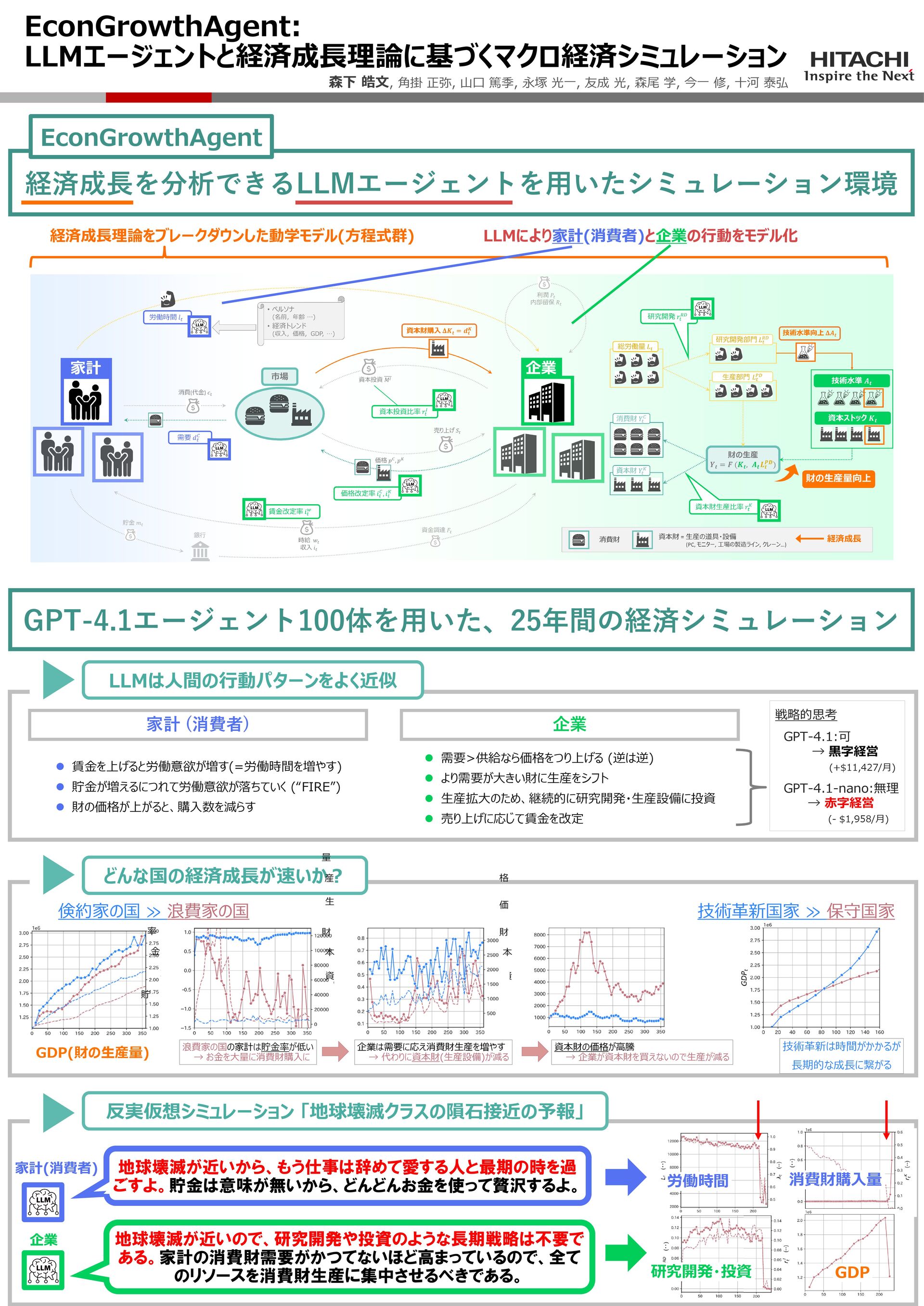
2. 3 EconGrowthAgent 127 Economic growth theory explains growth via two factors, “capital stock accumulation through 128 investment” and “technological innovation through R&D”, assuming given and fixed ratios for 129 investment (s) and R&D (r0). However, in reality, these factors arise from interactions among 130 micro-level decisions of economic agents, such as firms and households. Without this micro-level 131 lens, a comprehensive analysis of growth is impossible. 132 We therefore first break down growth theory into a system of dynamic equations describing how micro- 133 level decisions and other economic variables interact and evolve. We model capital accumulation 134 through a process where firms produce and sell capital goods, while other firms buy them to use in 135 their production. Similarly, we model technological innovation through firms allocating a portion 136 of labor to R&D, raising their technology levels. Furthermore, these decisions can be influenced by 137 those made within the same firms, as well as by other firms and households. For instance, funds for 138 purchasing capital goods come from previous sales, which depend on firm-set prices, competitors’ 139 prices, and household demand, while R&D labor depends on the labor supplied by households. Thus, 140 we enumerate a wide range of decision types for both firms and households, together with all relevant 141 interactions. 142 Then, we implement LLM agents to drive these dynamics with realistic decisions of households and 143 firms, creating an executable simulation environment named EconGrowthAgent (Figure 1). 144 3.1 LLM Agents 145 Assume NH household agents and NF firm agents. Each household h ∈ [1, NH] is assigned a 146 random persona prompt Pr(h)—including name, age, job, and residence—to approximate real-world 147 diversity. For decision-making, it receives a decision prompt DH listing decision items (e.g., “How 148 many goods to buy?”) and an economic trend prompt E(h) t providing variables up to timestep t 149 (month), such as income, goods prices and previous consumption, to support rational decisions. 150 For counterfactual simulations, it receives a counterfactual prompt Ct (e.g., “a novel infection X is 151 spreading”). We concatenate these into a single prompt PH(h) t = Pr(h) ⊕ DH ⊕ E(h) t ⊕ Ct to query 152 LLMs. 153 Likewise, each firm f ∈ [1, NF ] receives PF (f) t = Pr(f) ⊕ DF ⊕ E(f) t ⊕ Ct. E(f) t includes 154 firm-related variables (e.g., past demand and sales). See Appendix E for the details and LLM outputs. 155 4
3. 3.2 Household Equations 156 ▶ Labor and Income: The household h determines their working hours. This labor is provided to 157 their employer (discussed later), and the household receives income for the month as compensation: 158 labor hours l(h) t = LLM(PH(h) t ) monthly income i(h) t = w(h) t × l(h) t (7) w(h) t is the hourly wage. LLM decisions are shown in blue. 159 ▶ Consumption and Savings: The household determines the quantity of consumer goods to purchase 160 (i.e., demand), and purchases from the firm σH t = argminf pC(f) t offering the lowest price pC(f) t : 161 quantity of consumer goods purchased (i.e., demand) dC(h)→(σH t ) t = LLM(PH(h) t ) (8) consumption expenditure c(h) t = dC(h)→(σH t ) t × pC(σH t ) t (9) After paying for the company, the household deposits the remainder in the bank (Appendix F.1.1). 162 3.3 Firm Equations 163 Firm decision variables are shown in green. 164 ▶ Labor Allocation Between Departments: The firm f allocates labor from its employees E(f) ⊂ 165 {1, . . . , NH}, a a random subset of households, between production and R&D department: 166 total labor L(f) t = h∈E(f) l(h) t R&D ratio rRD(f) t = LLM(PF (f) t ) (10) R&D labor LRD(f) t = rRD(f) t × L(f) t production labor LP D(f) t = (1 − rRD(f) t ) × L(f) t (11) ▶ Production of Goods by Production Department: The firm sets the production ratio of consumer 167 and capital goods within its total production, constrained by the Cobb–Douglas function F eq. (2): 168 total production Y (f) t = F(K(f) t , A(f) t LP D(f) t ) capital goods production ratio rK(f) t = LLM(PF (f) t ) (12) consumer goods production Y C(f) t = (1 − rK(f) t ) × Y (f) t capital goods production Y K(f) t = rK(f) t × Y (f) t Here, K(f) t is firm f’s capital stock, and A(f) t its technology level. 169 ▶ Technological Innovation by R&D Department: 170 A(f) t+1 = A(f) t + ∆A(f) t (13) The growth ∆A(f) t depends on R&D labor LRD t and the delay (i.e., the time until R&D yields results) 171 τRD before results (Appendix F.2.1). 172 ▶ Setting Prices of Goods: 173 consumer goods price change rate iC(f) t = LLM(PF (f) t ) capital goods price change rate iK(f) t = LLM(PF (f) t ) consumer goods price pC(f) t+1 = (1 + iC(f) t ) × pC(f) t capital goods price pK(f) t+1 = (1 + iK(f) t ) × pK(f) t ▶ Sales of Goods: The firm sells consumer goods to households and capital goods to other firms: 174 consumer goods sales SC(f) t = pC(f) t × DC(f) t demand DC(f) t = h∈[1,Nh] dC(h)→(f) t (14) capital goods sales SK(f) t = pK(f) t × DK(f) t demand DK(f) t = f′∈[1,NF ] dK(f′)→(f) t (15) The goods inventories V C(f) t , V K(f) t are updated depending on the sales volume (Appendix F.2.2). 175 ▶ Wage Revision: The firm can revise employees’ wages, e.g., to boost motivation or reduce cost: 176 wage change rate iw(h) t = LLM(PF (f) t ) employee wage w(h) t+1 = (1 + iw(h) t ) × w(h) t (h ∈ E(f)) ▶ Wage Payment: The firm pays employee wages (i.e., personnel cost) from sales plus bank 177 financing Ft (Appendix F.3): 178 total sales S(f) t = SC(f) t + SK(f) t personnel cost C(f) t = h∈E(f) i(h) t = h∈E(f) w(h) t × l(h) t remaining funds M(f) t = S(f) t + F(f) t − C(f) t ▶ Capital Stock Accumulation by Capital Goods Purchase: The firm can purchase capital goods 179 to expand future production (capital investment). Within its budget of M(f) t plus retained earnings 180 R(f) t , the firm buys from the lowest-price firm σF t = argminf′ pK(f′) t : 181 capital investment ratio rI(f) t = LLM(PF (f) t ) investment funds MI(f) t = rI(f) t × (M(f) t + R(f) t ) (16) quantity of capital goods purchased (demand) dK(f)→(σF t ) t = ⌊MI(f) t /pK(σF t ) t ⌋ (17) The purchased goods are added to the capital stock and used in production from the next period: 182 K(f) t+1 = K(f) t + dK(f)→(σF t ) t (18) Note that the capital goods production ratio rK(f) t eq. (12) capital investment ratio and rI(f) t here are 183 completely different. The former determines how many capital goods to produce for sale to other 184 firms, while the latter determines how many to purchase for use in one’s own production. 1 185 1 As we assume for simplicity that “only one type of capital good exists,” it may seem strange that capital goods production ratio and capital investment ratio differ. However, in the real world, these two are definitely different: a firm producing and selling “food processing lines” does not use food processing lines by themselves. 5