I gave 3-hours of lectures at the Asteroseismology and Exoplanets: Listening to the Stars and Searching for New Worlds, at the IVth Azores International Advanced School in Space Sciences. Here are the sldies
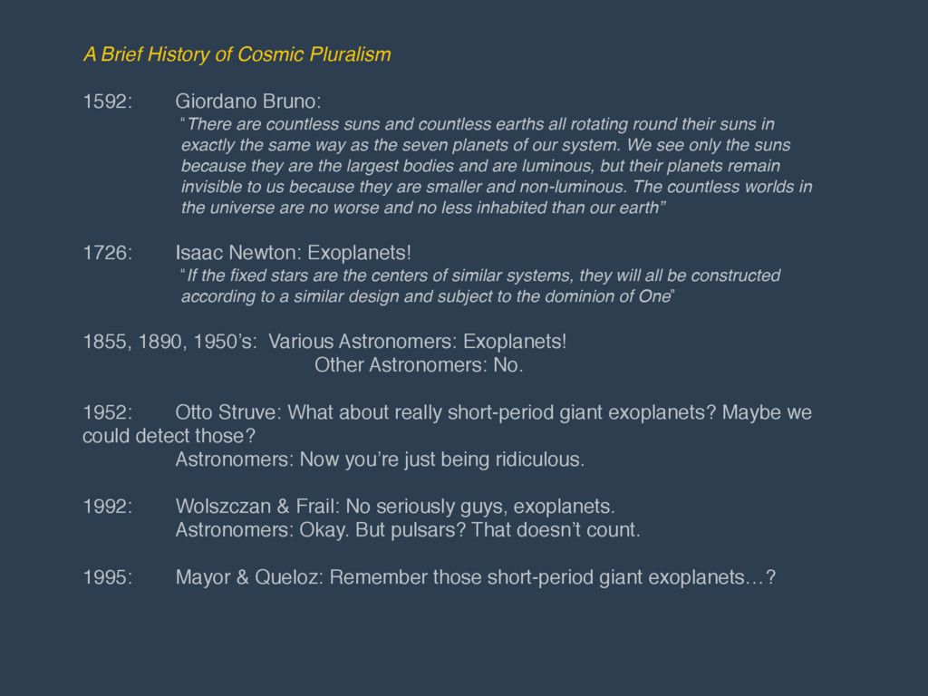
are countless suns and countless earths all rotating round their suns in exactly the same way as the seven planets of our system. We see only the suns because they are the largest bodies and are luminous, but their planets remain invisible to us because they are smaller and non-luminous. The countless worlds in the universe are no worse and no less inhabited than our earth” 1726: Isaac Newton: Exoplanets! “If the fixed stars are the centers of similar systems, they will all be constructed according to a similar design and subject to the dominion of One” 1855, 1890, 1950’s: Various Astronomers: Exoplanets! Other Astronomers: No. 1952: Otto Struve: What about really short-period giant exoplanets? Maybe we could detect those? Astronomers: Now you’re just being ridiculous. 1992: Wolszczan & Frail: No seriously guys, exoplanets. Astronomers: Okay. But pulsars? That doesn’t count. 1995: Mayor & Queloz: Remember those short-period giant exoplanets…?
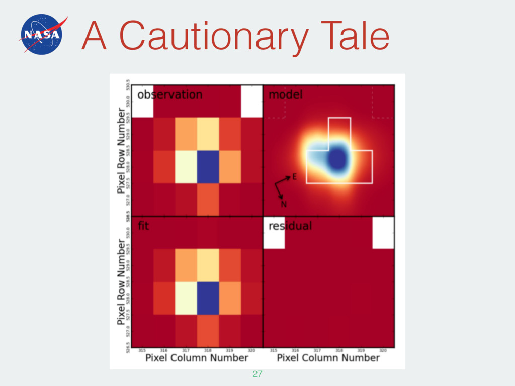
comes from eclipsing systems, even after more than a century since eclipses were first observed. The same is likely to be true for exoplanets. Josh Winn 5
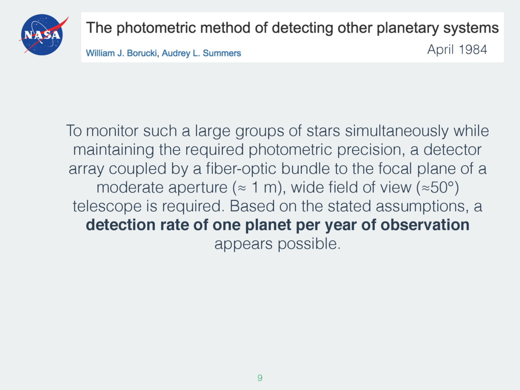
maintaining the required photometric precision, a detector array coupled by a fiber-optic bundle to the focal plane of a moderate aperture (≈ 1 m), wide field of view (≈50°) telescope is required. Based on the stated assumptions, a detection rate of one planet per year of observation appears possible. 9 April 1984
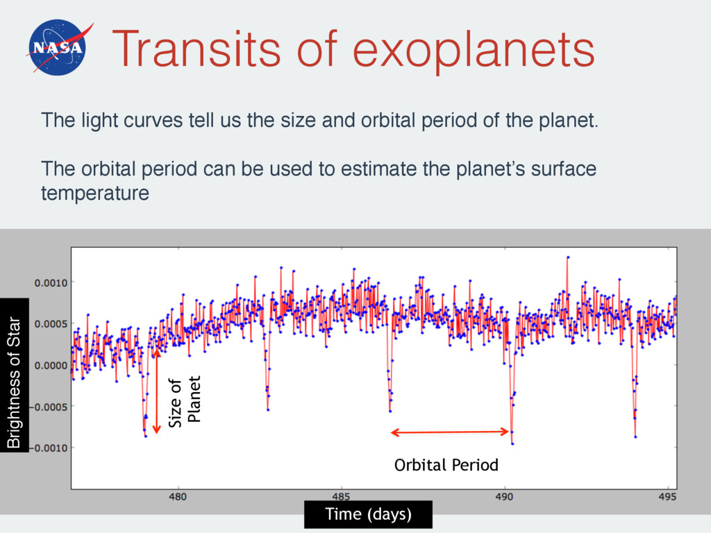
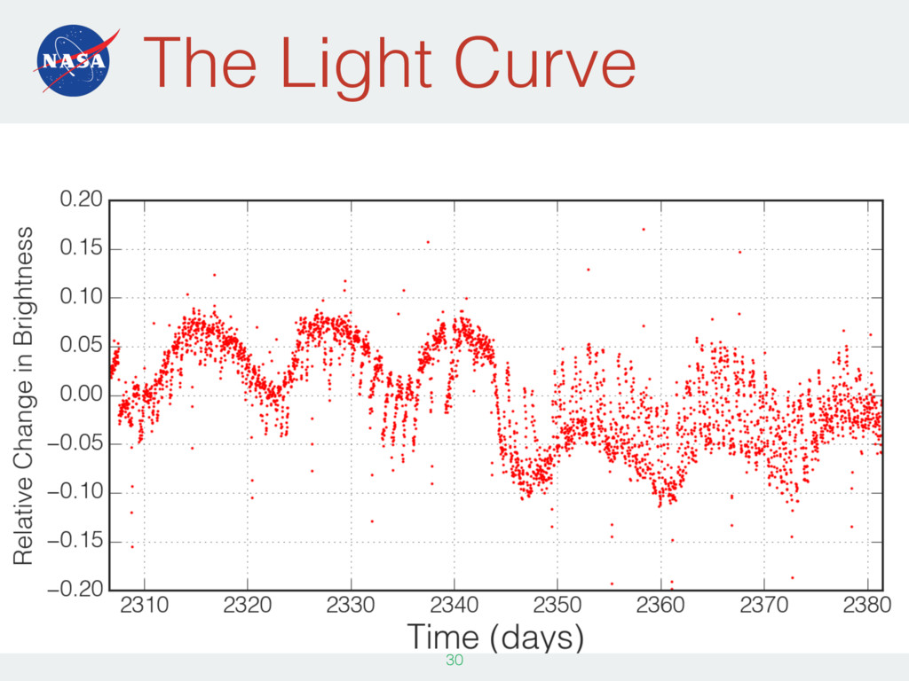
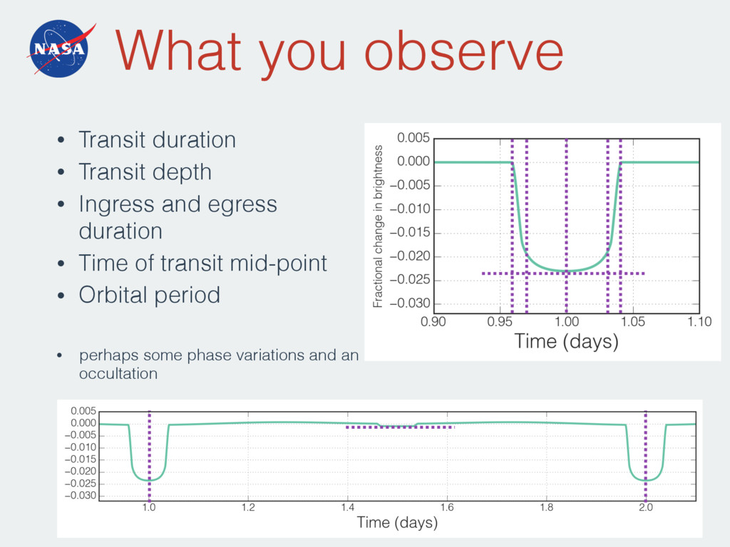
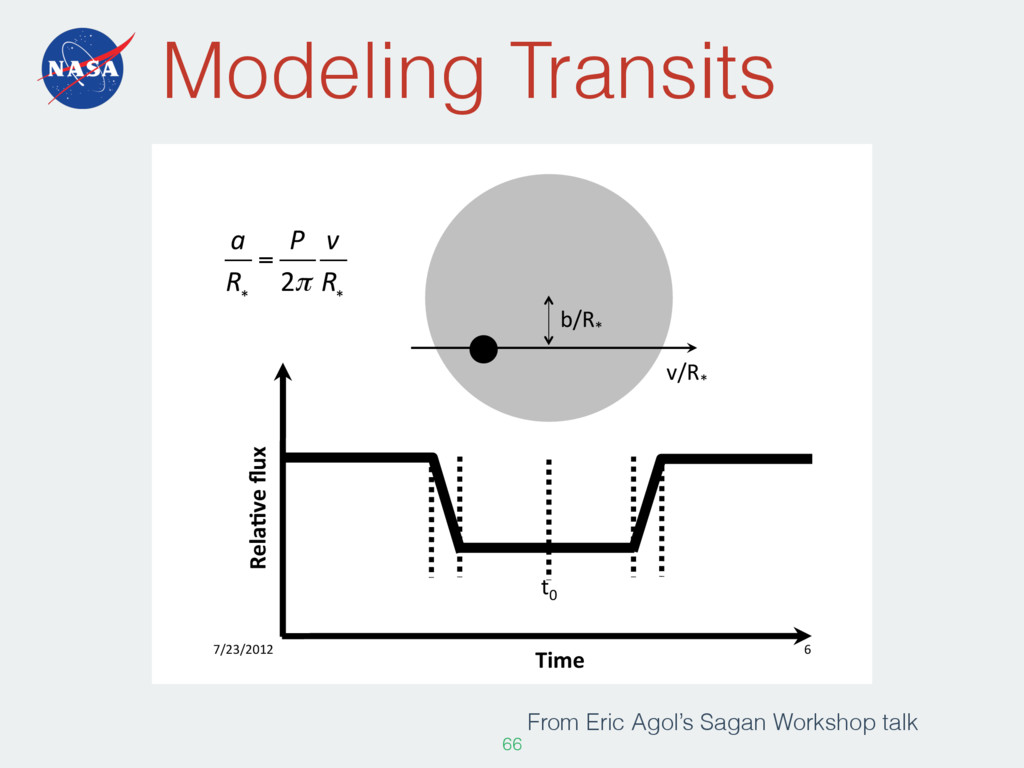
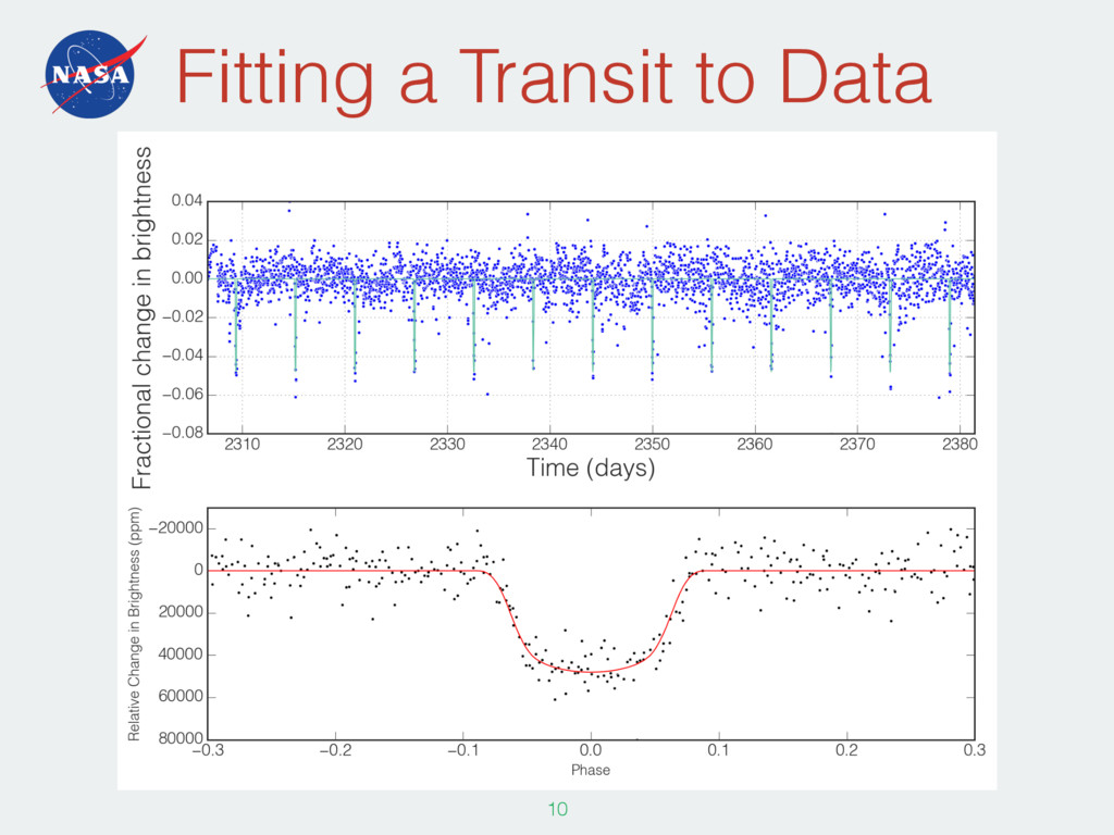
light curves tell us the size and orbital period of the planet. The orbital period can be used to estimate the planet’s surface temperature Brightness of Star Time (days)
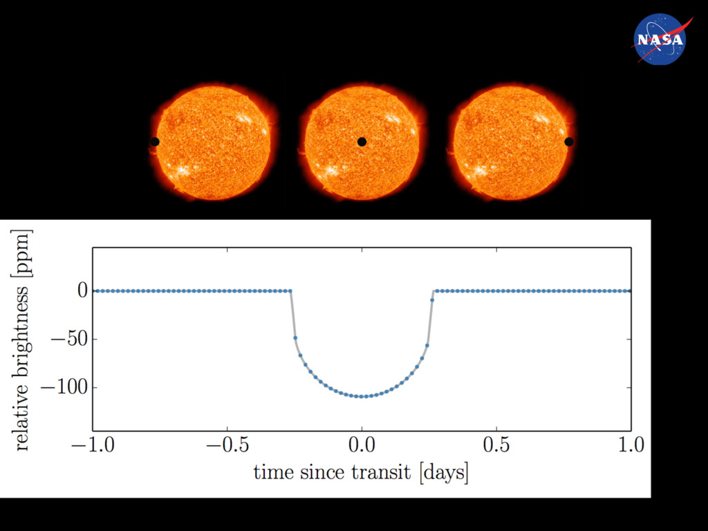
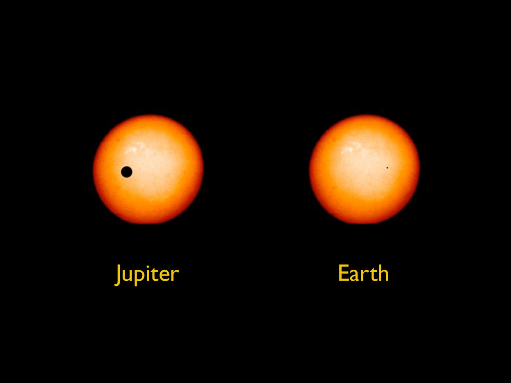
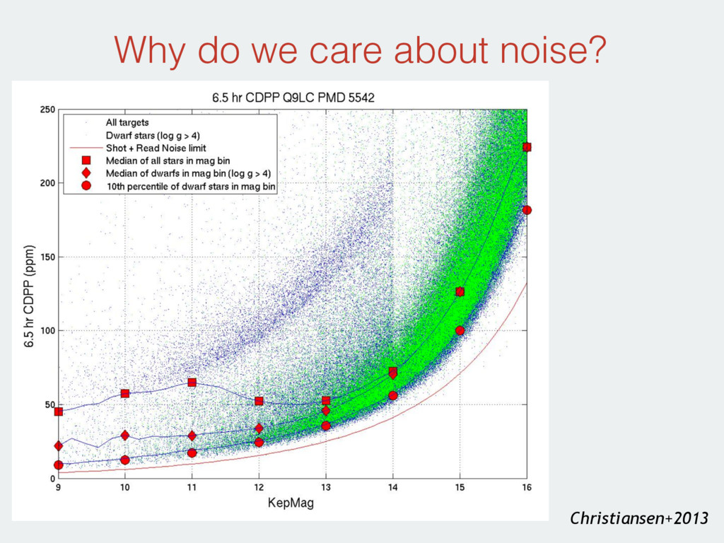
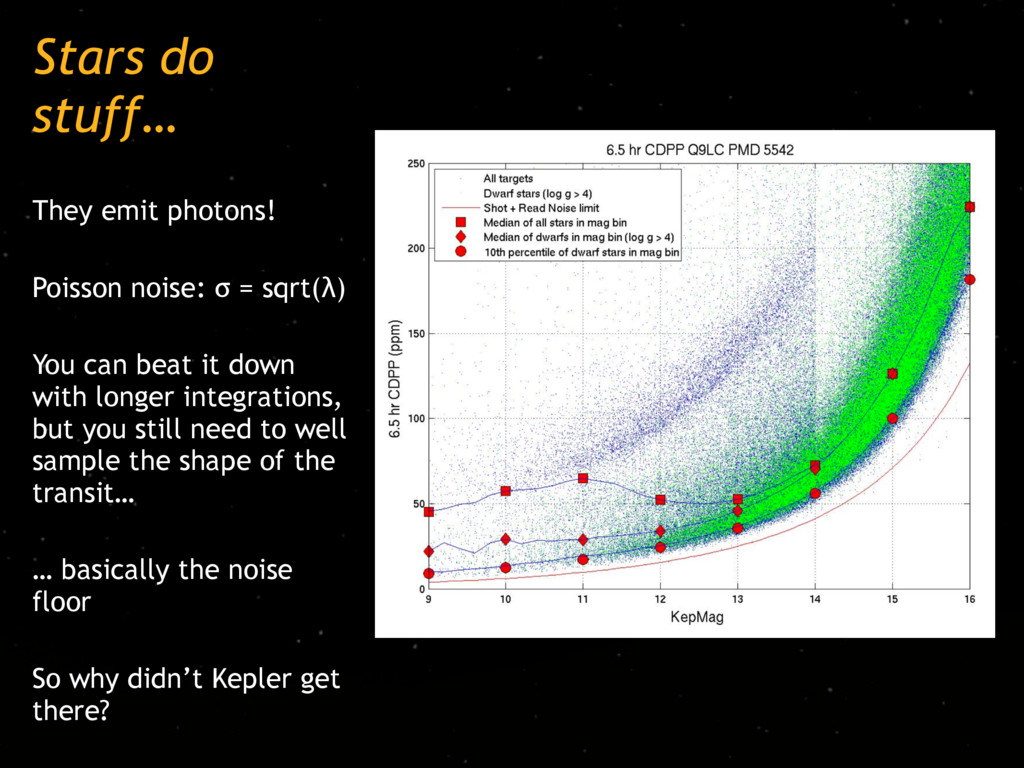
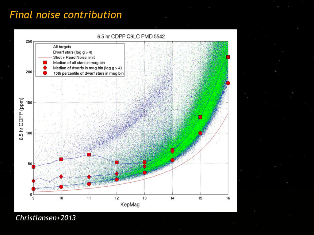
goal was measuring the occurrence rate of Earth-like planets around sunlike stars That’s hard! Earth has an 85ppm transit Design needed to account for all known sources of noise – budget of 20ppm in 6h at Kp=12 Stars (10ppm), Poisson (14ppm), Detector (10ppm) How big a telescope do we need? How faint a star can we look at? How much do we need to spend on a detector? Christiansen+2013 Why do we care about noise?
sqrt(λ) You can beat it down with longer integrations, but you still need to well sample the shape of the transit… … basically the noise floor So why didn’t Kepler get there?
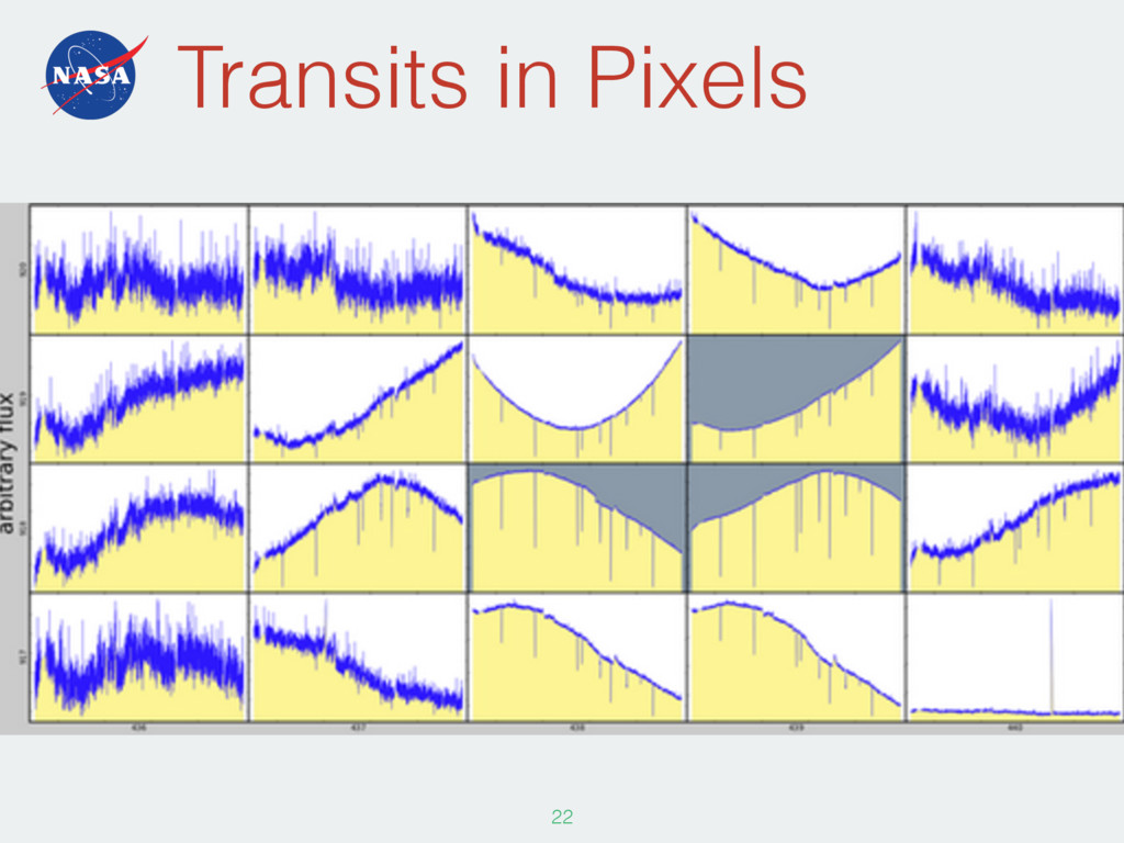
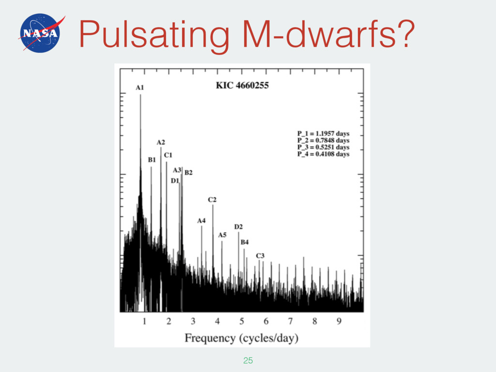
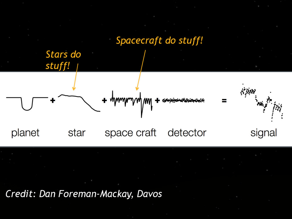
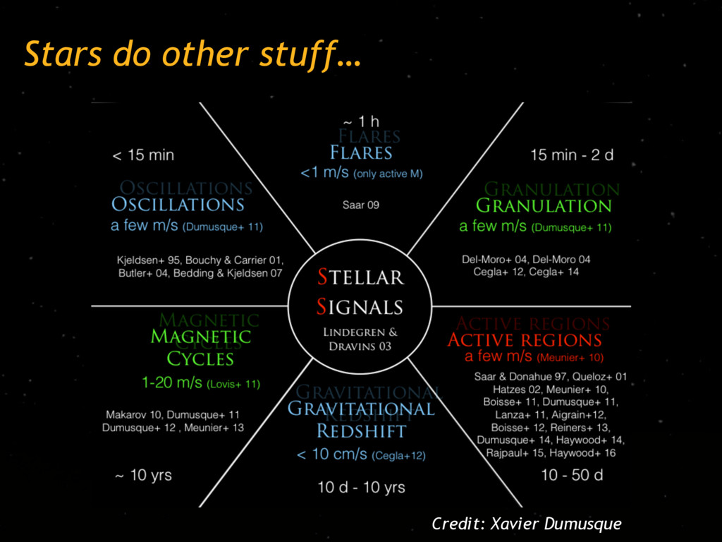
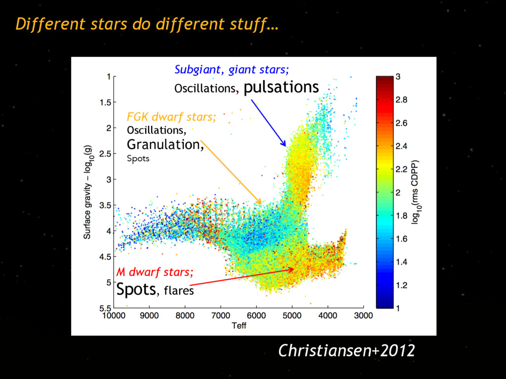
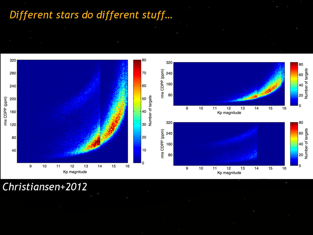
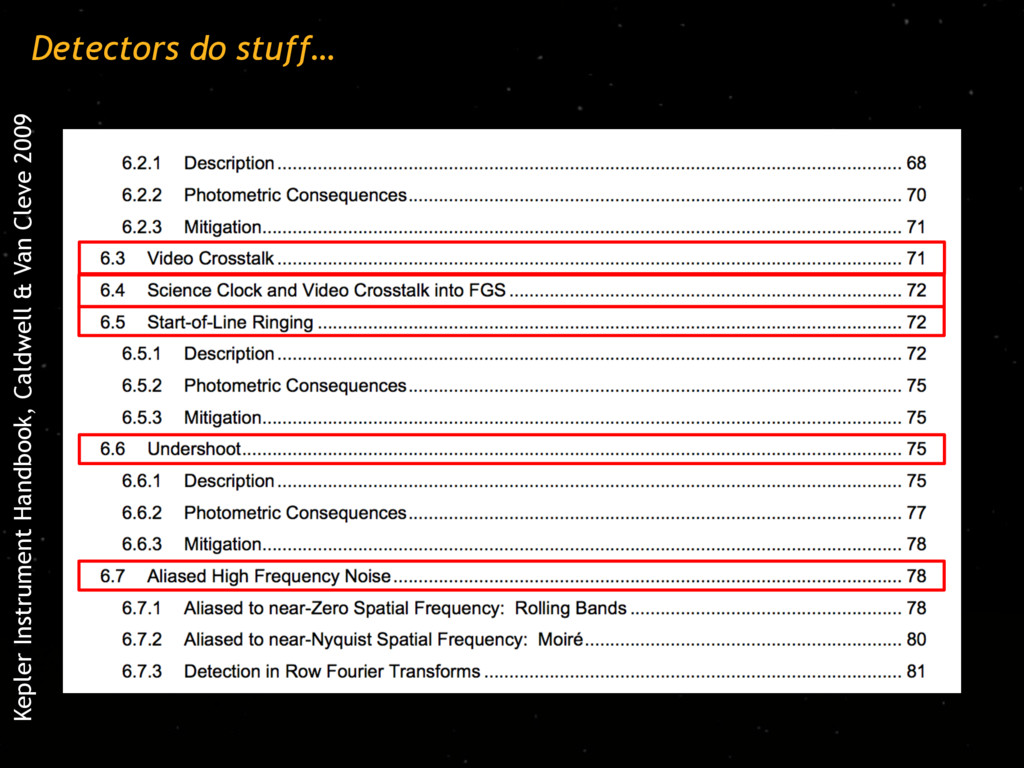
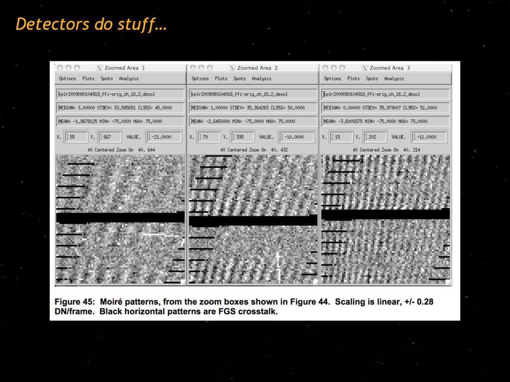
(2days to weeks, <10%)) - flares (stochastic,<few%) Pulsations (mins to yrs, <10s of %) Eclipses (hrs to yrs, <50%) Yikes! Luckily, we are mostly saved by timescales and careful target selection Stars do stuff… Credit: Arcetri Solar Physics Group/NSO Paz-Chinchon+2015 Credit: NASA/SDO Davenport et al. 2014 Molner+2014 Christiansen, PhD thesis, 2007
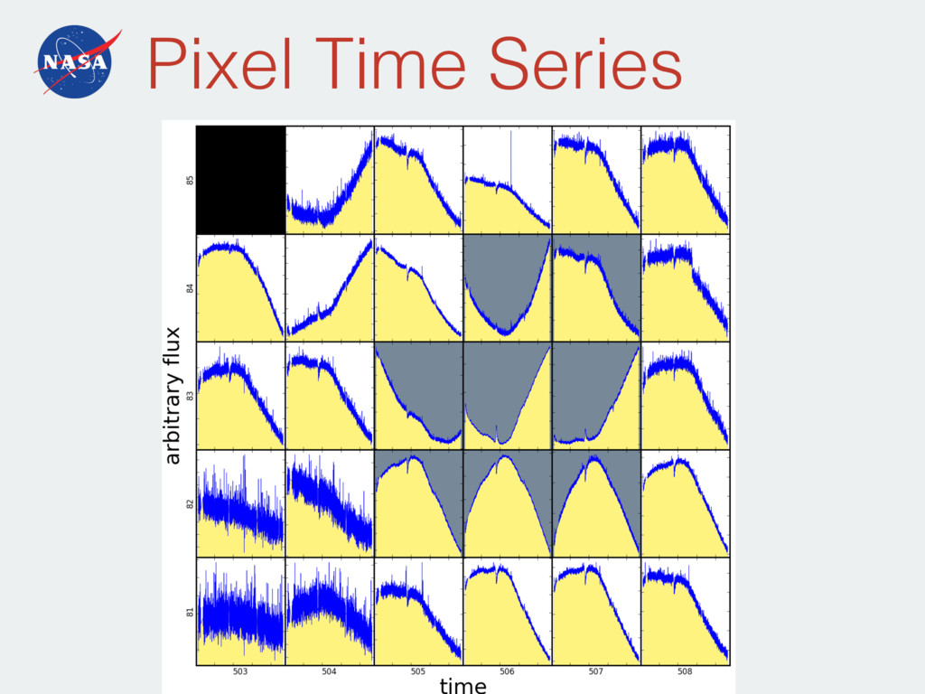
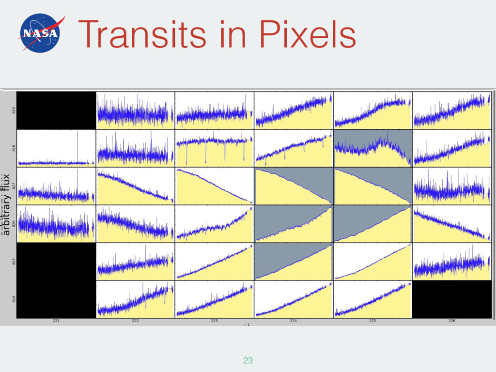
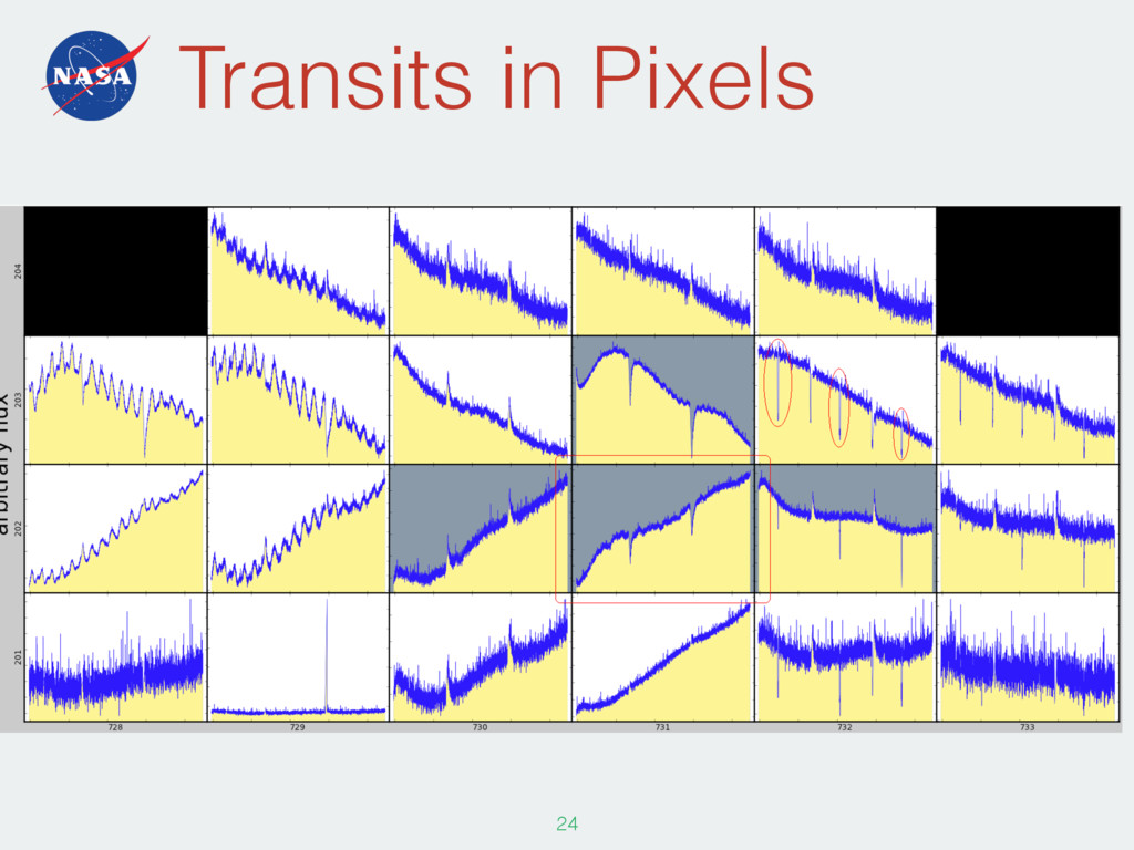
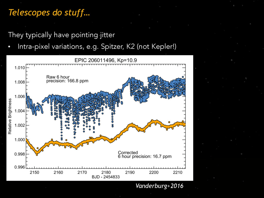
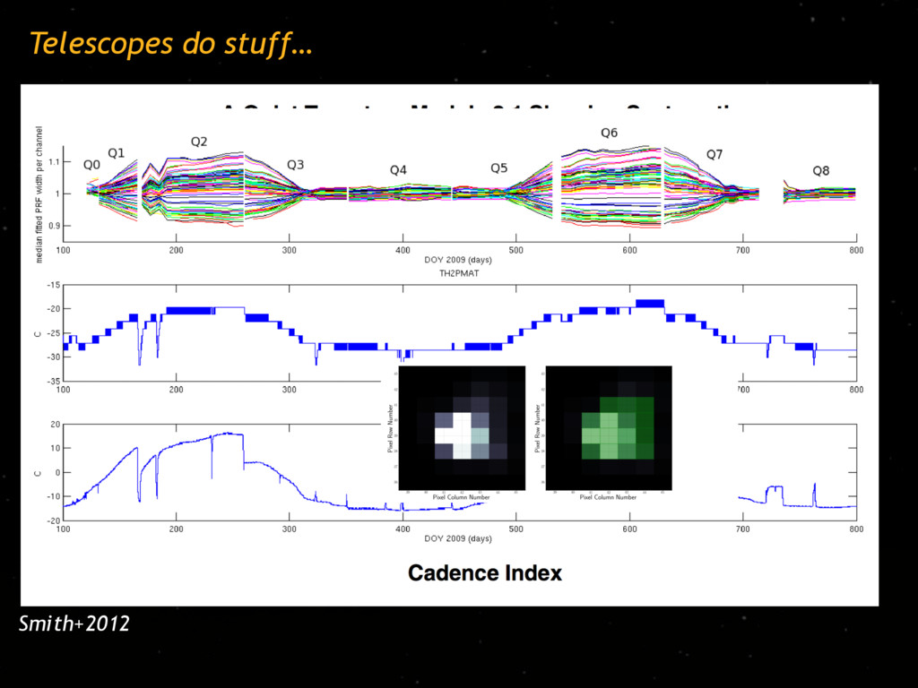
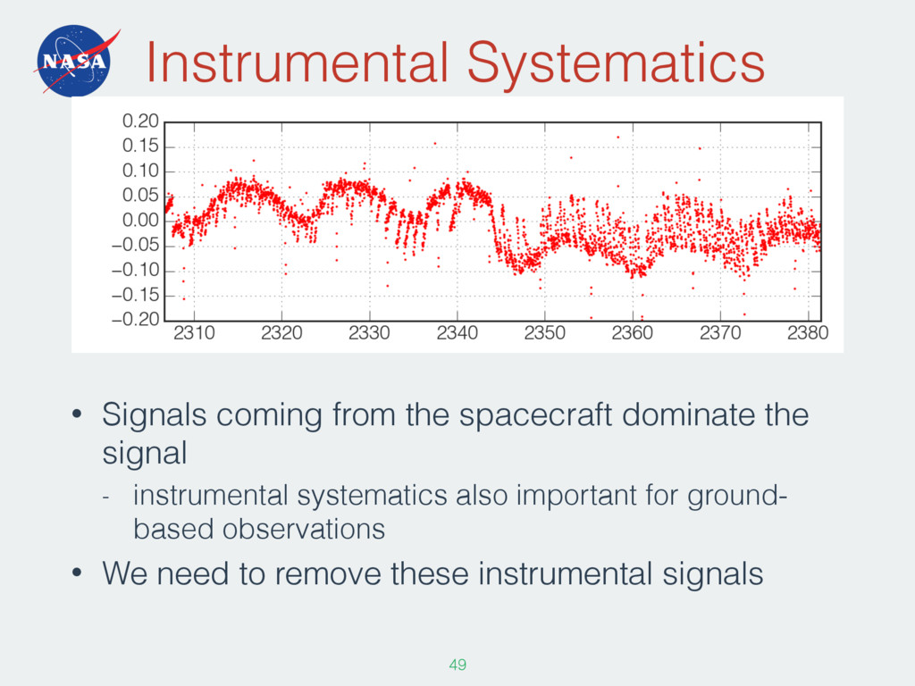
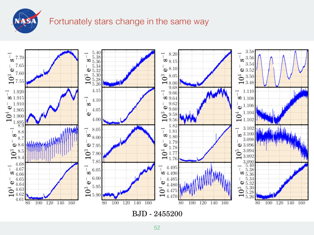
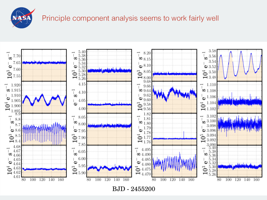
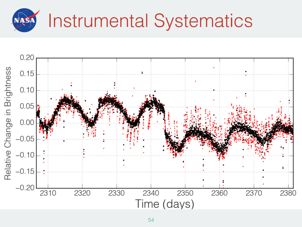
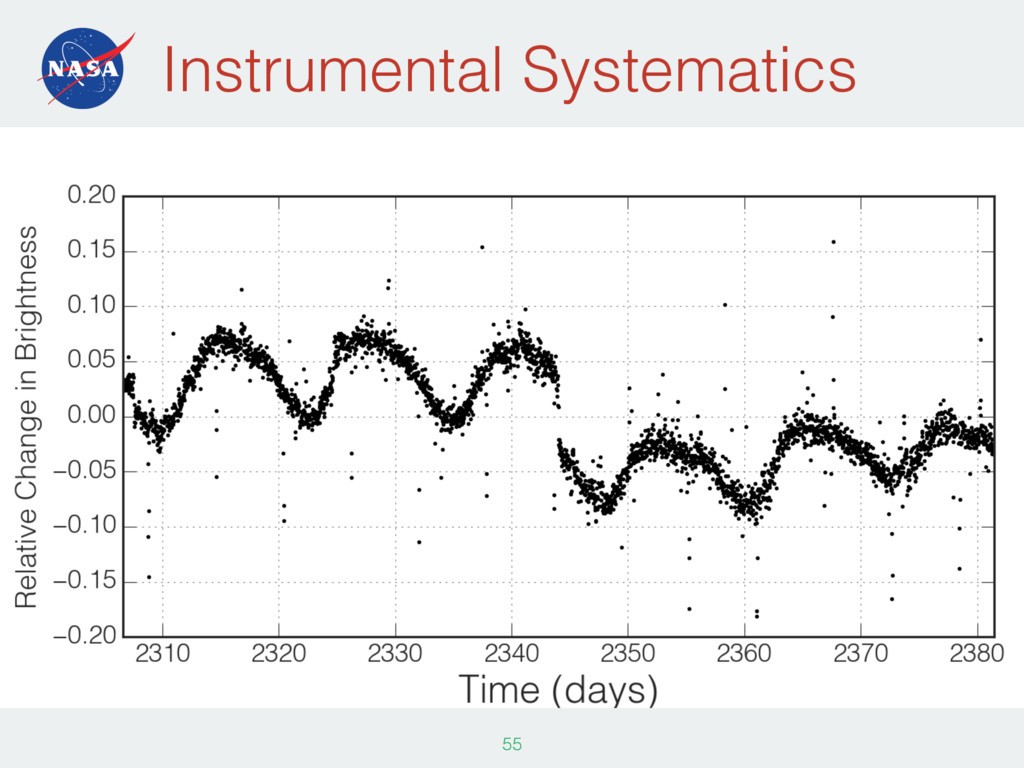
K2 (not Kepler!) • Inter-pixel variations, e.g. EPOCh They experience thermal variations, e.g. Kepler Telescopes do stuff… Smith+2012 Christiansen+2013
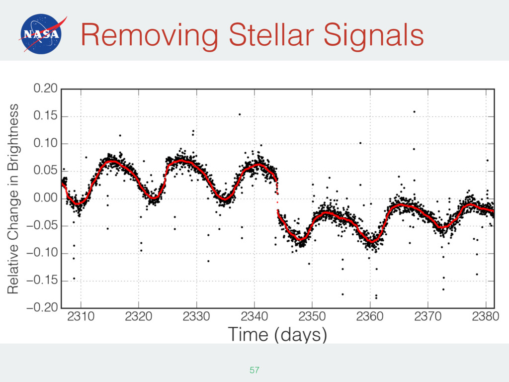
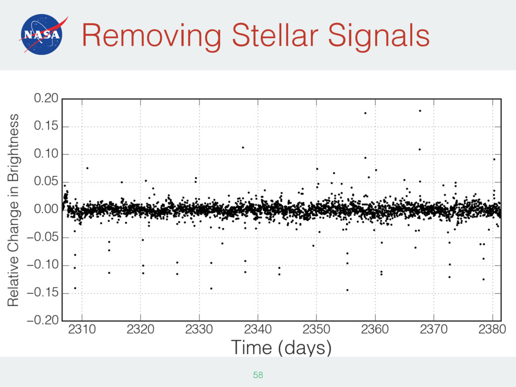
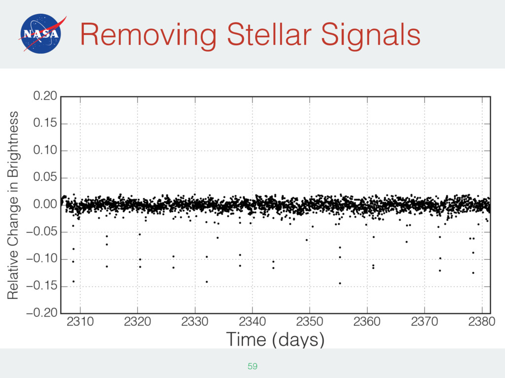
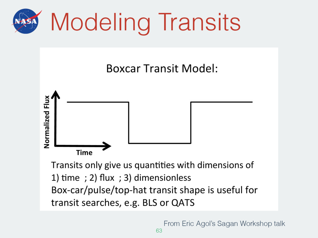
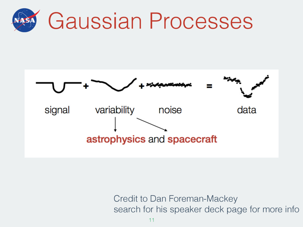
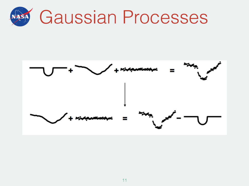
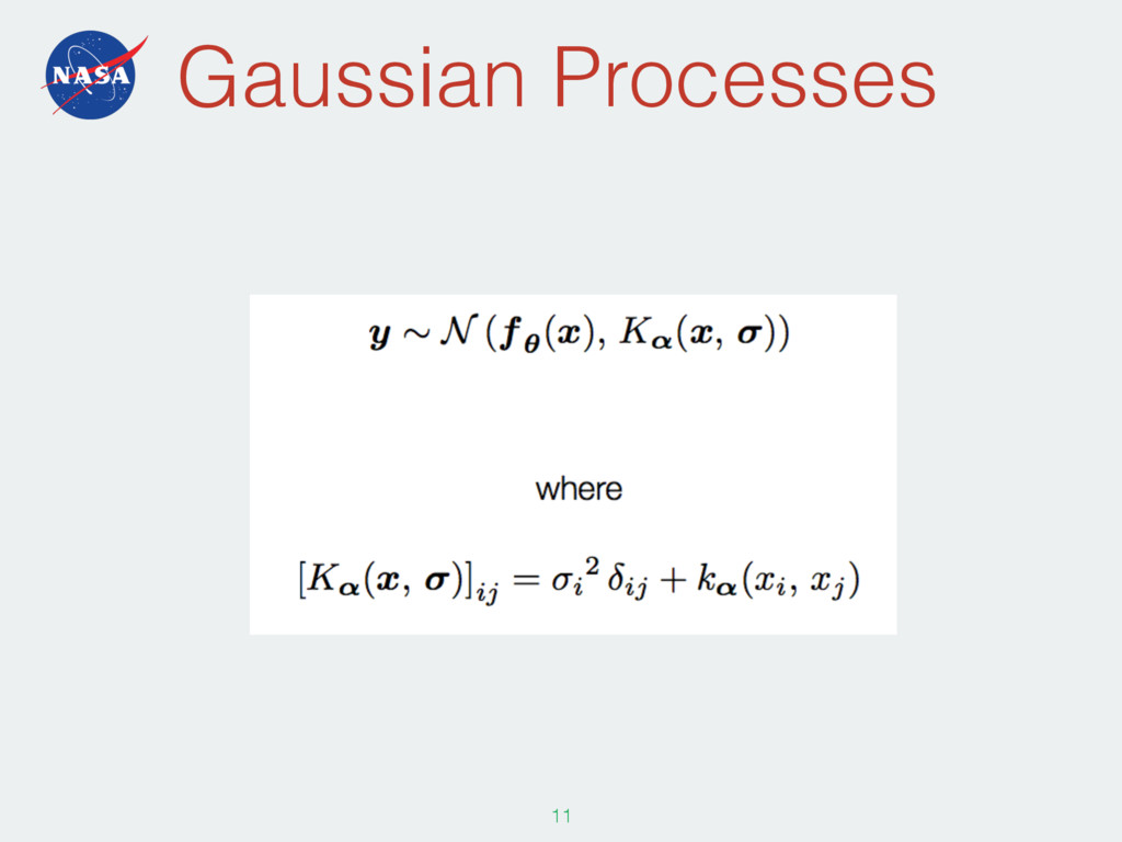
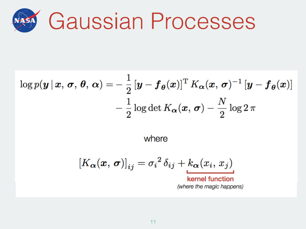
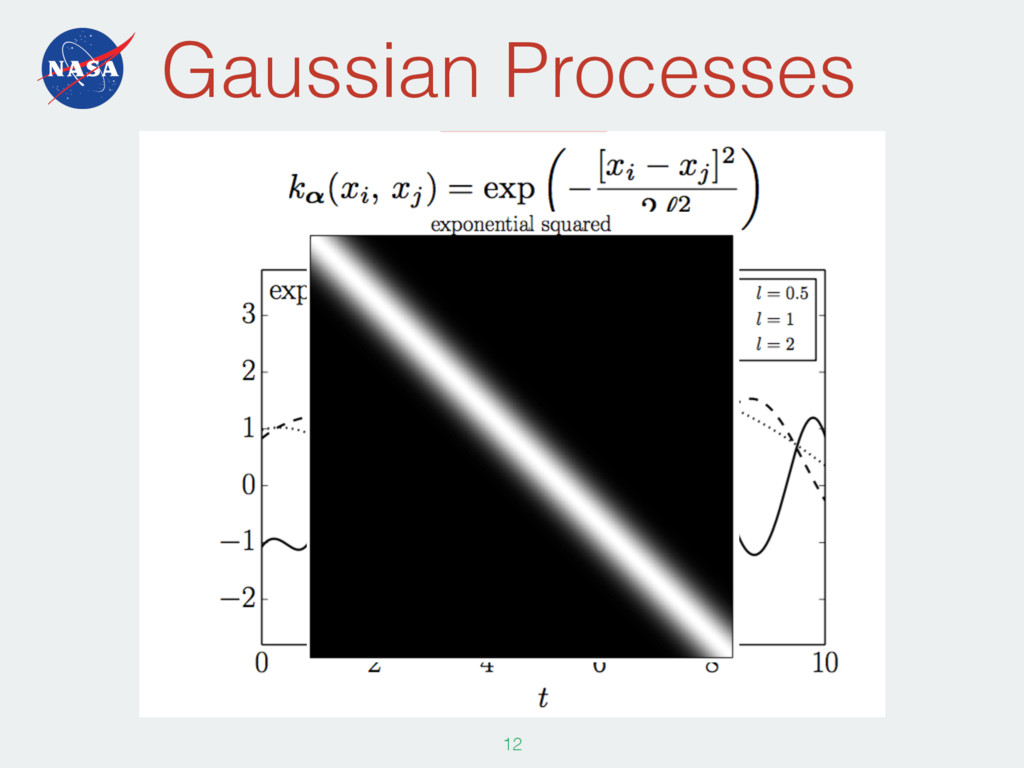
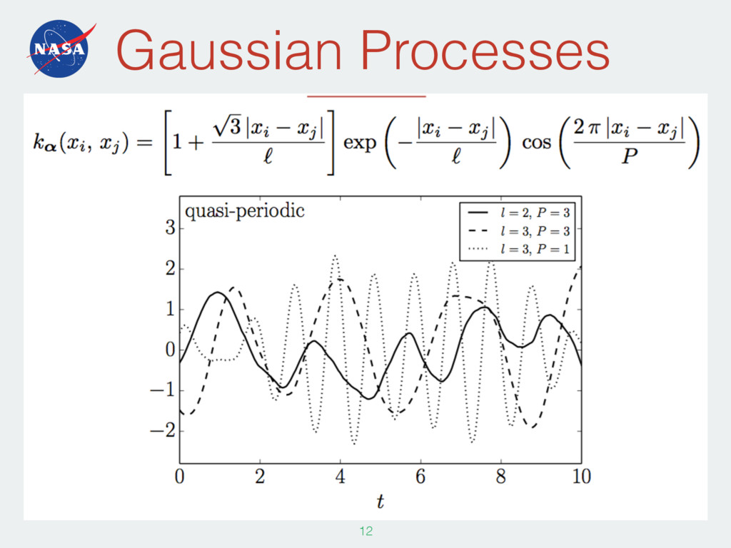
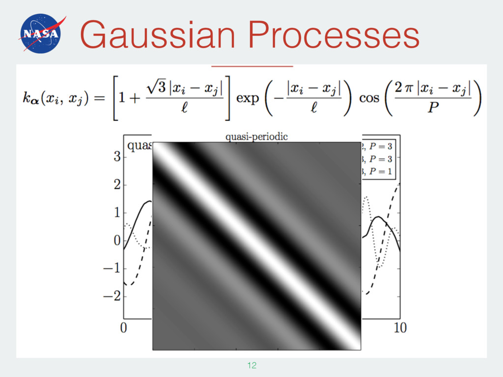
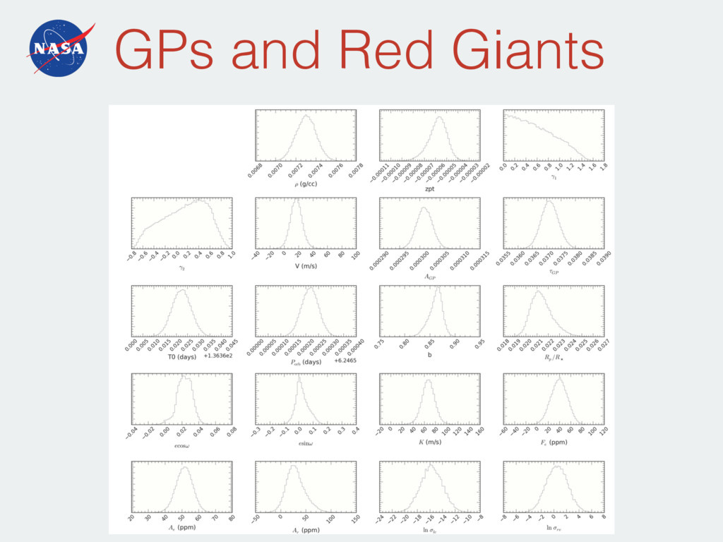
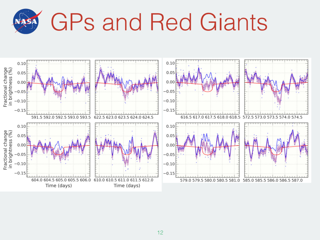
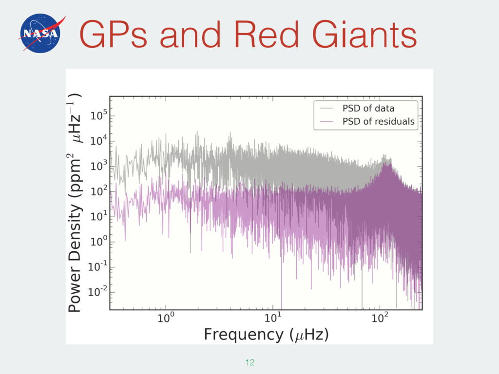
filter - not always (ever?) a good choice but often good enough - masking transits is always a good idea - better alternatives are using a locally conditioned function (i.e. polynomial, spline, etc.) • The right way is to build a physical model • Later on I’ll mention Gaussian Processes 56
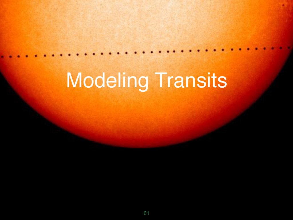
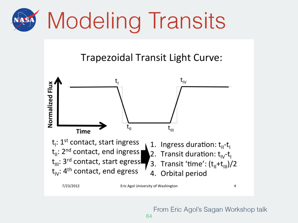
Normalized+Flux+ Time+ t I :'1st'contact,'start'ingress' t II :'2nd'contact,'end'ingress' t III :'3rd'contact,'start'egress' t IV :'4th'contact,'end'egress' 1. Ingress'duraJon:'t II Nt I ' 2. Transit'duraJon:'t IV Nt I '' 3. Transit'‘Jme’:'(t II +t III )/2' 4. Orbital'period' t I t II t III t IV From Eric Agol’s Sagan Workshop talk
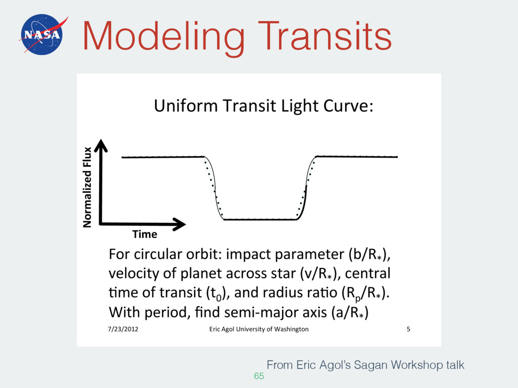
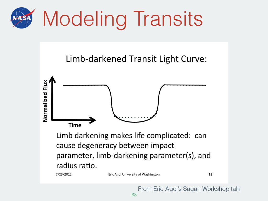
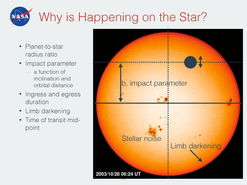
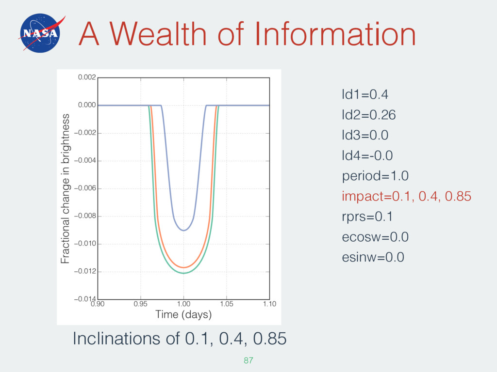
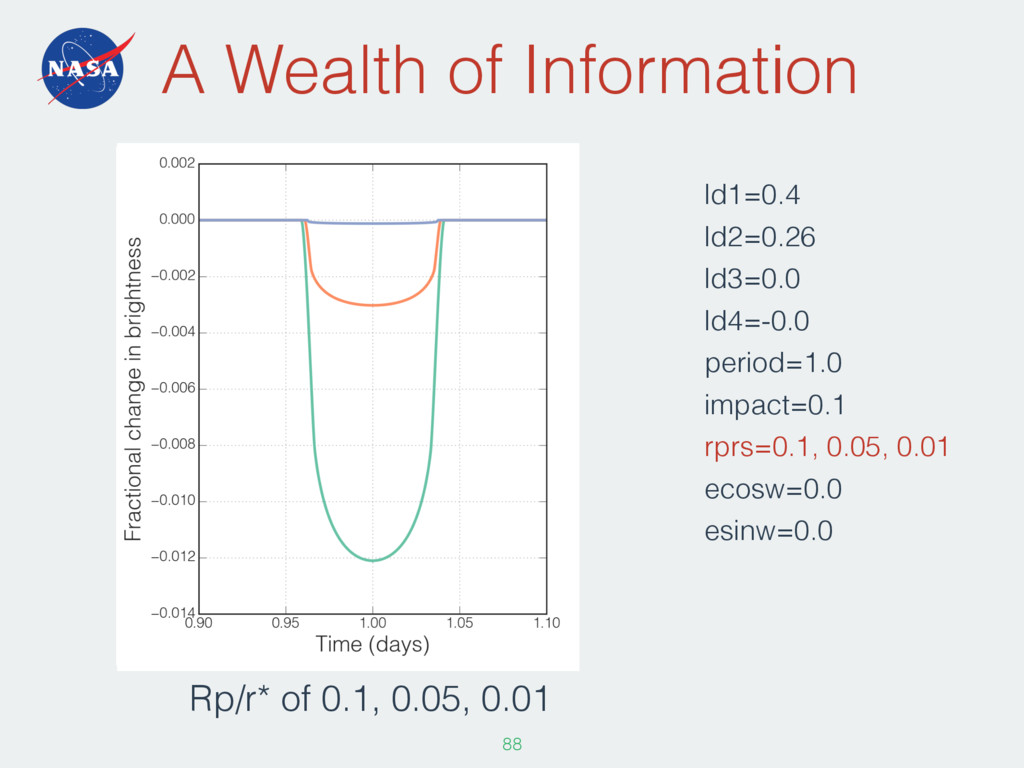
• Planet-to-star radius ratio • Impact parameter - a function of inclination and orbital distance • Ingress and egress duration • Limb darkening • Time of transit mid- point Limb darkening Stellar noise
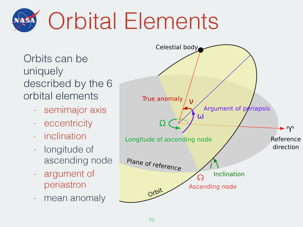
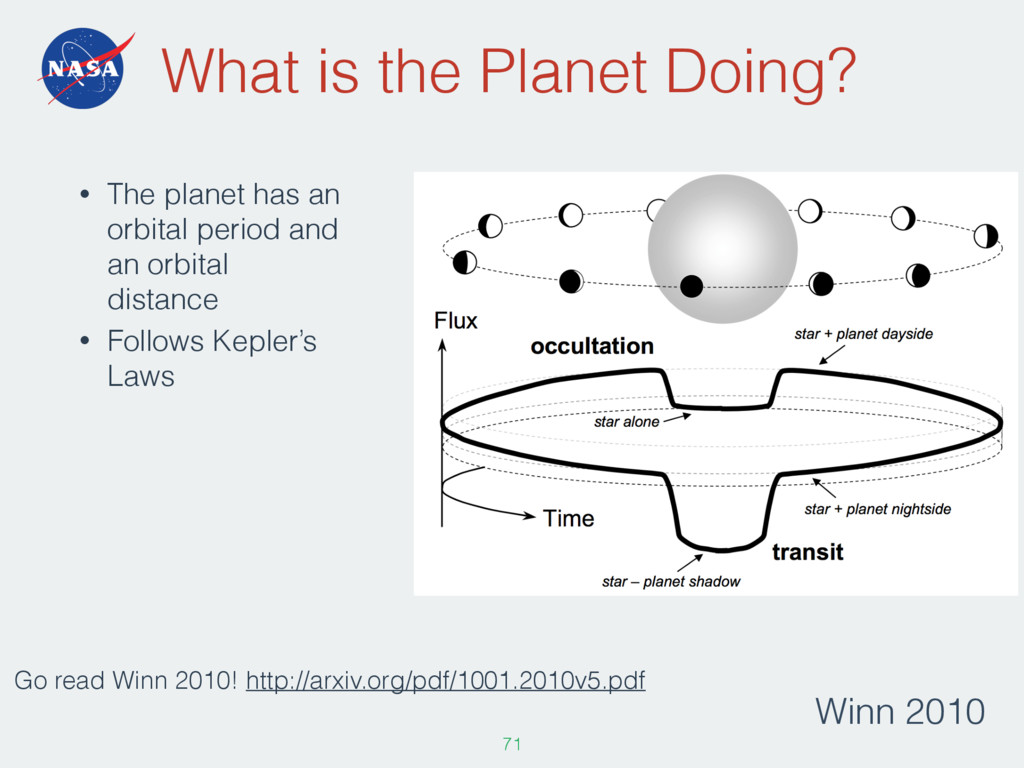
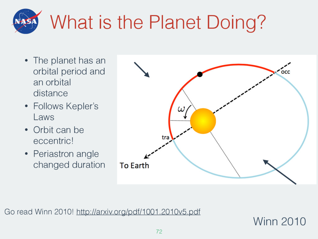
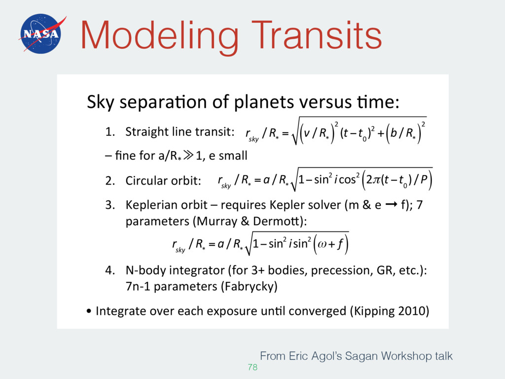
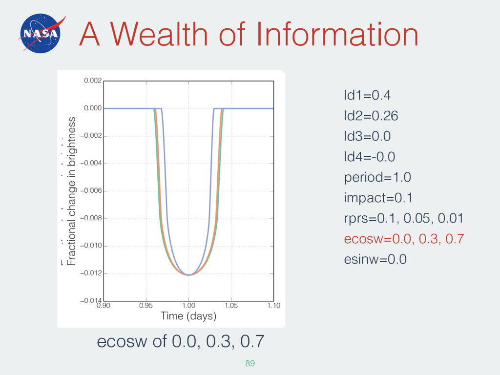
planet has an orbital period and an orbital distance • Follows Kepler’s Laws • Orbit can be eccentric! • Periastron angle changed duration Go read Winn 2010! http://arxiv.org/pdf/1001.2010v5.pdf
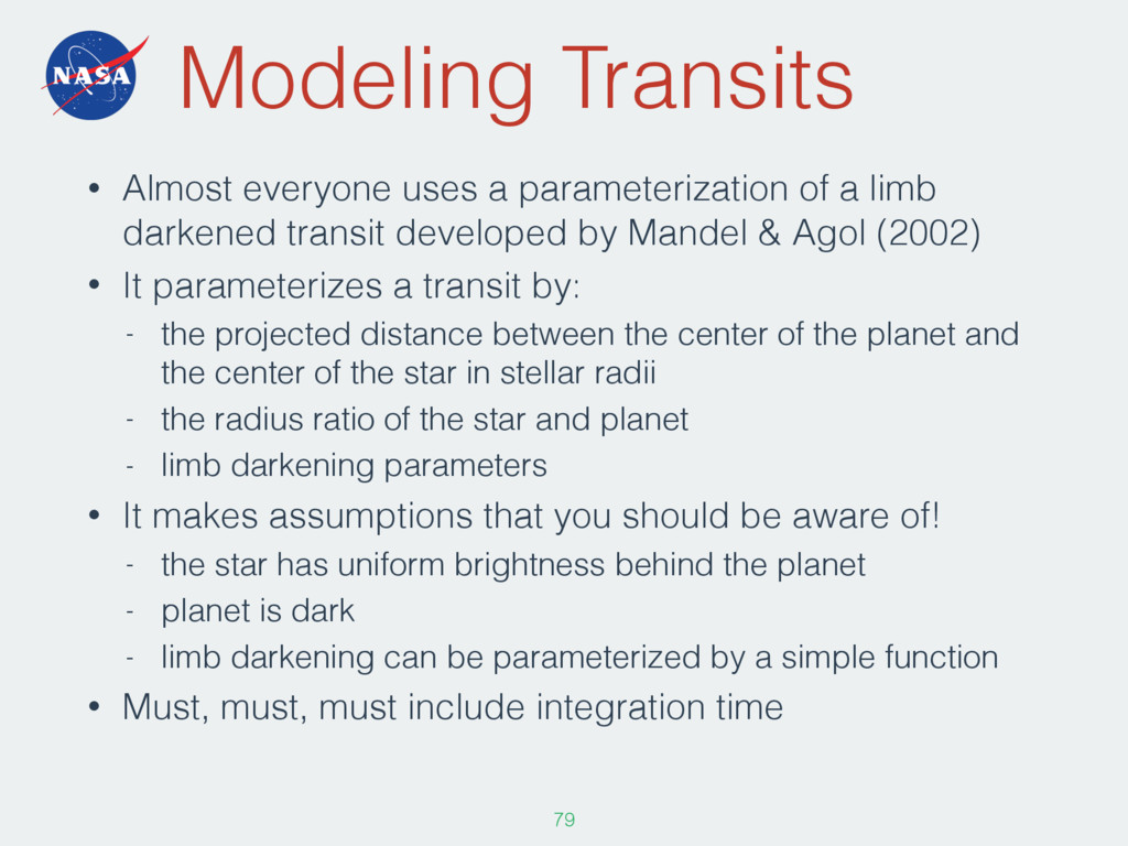
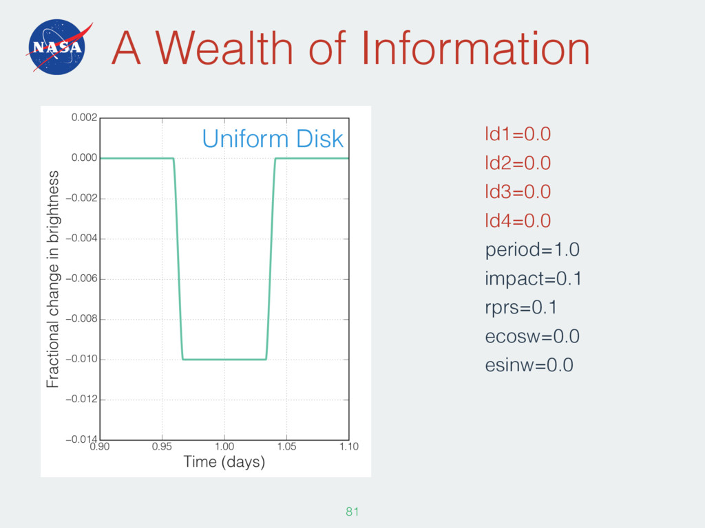
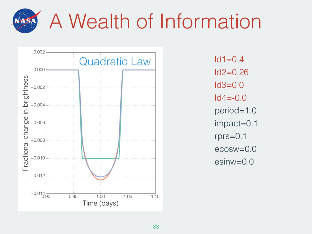
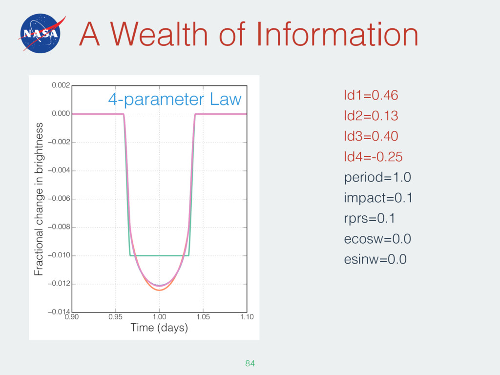
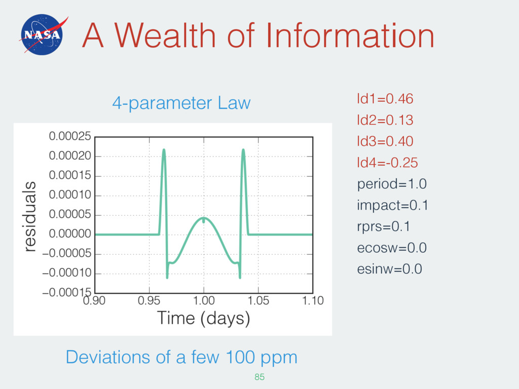
limb darkened transit developed by Mandel & Agol (2002) • It parameterizes a transit by: - the projected distance between the center of the planet and the center of the star in stellar radii - the radius ratio of the star and planet - limb darkening parameters • It makes assumptions that you should be aware of! - the star has uniform brightness behind the planet - planet is dark - limb darkening can be parameterized by a simple function • Must, must, must include integration time 79
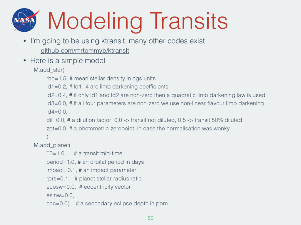
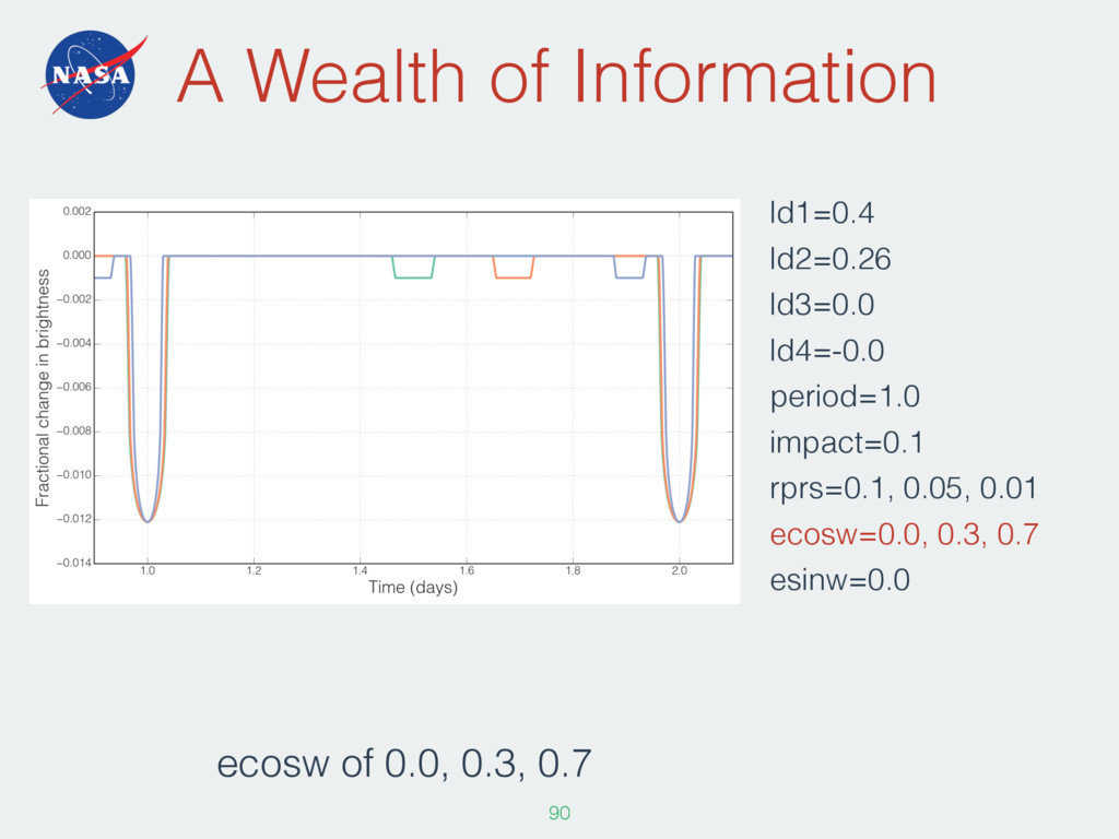
other codes exist - github.com/mrtommyb/ktransit • Here is a simple model M.add_star( rho=1.5, # mean stellar density in cgs units ld1=0.2, # ld1--4 are limb darkening coefficients ld2=0.4, # if only ld1 and ld2 are non-zero then a quadratic limb darkening law is used ld3=0.0, # if all four parameters are non-zero we use non-linear flavour limb darkening ld4=0.0, dil=0.0, # a dilution factor: 0.0 -> transit not diluted, 0.5 -> transit 50% diluted zpt=0.0 # a photometric zeropoint, in case the normalisation was wonky ) M.add_planet( T0=1.0, # a transit mid-time period=1.0, # an orbital period in days impact=0.1, # an impact parameter rprs=0.1, # planet stellar radius ratio ecosw=0.0, # eccentricity vector esinw=0.0, occ=0.0) # a secondary eclipse depth in ppm 80
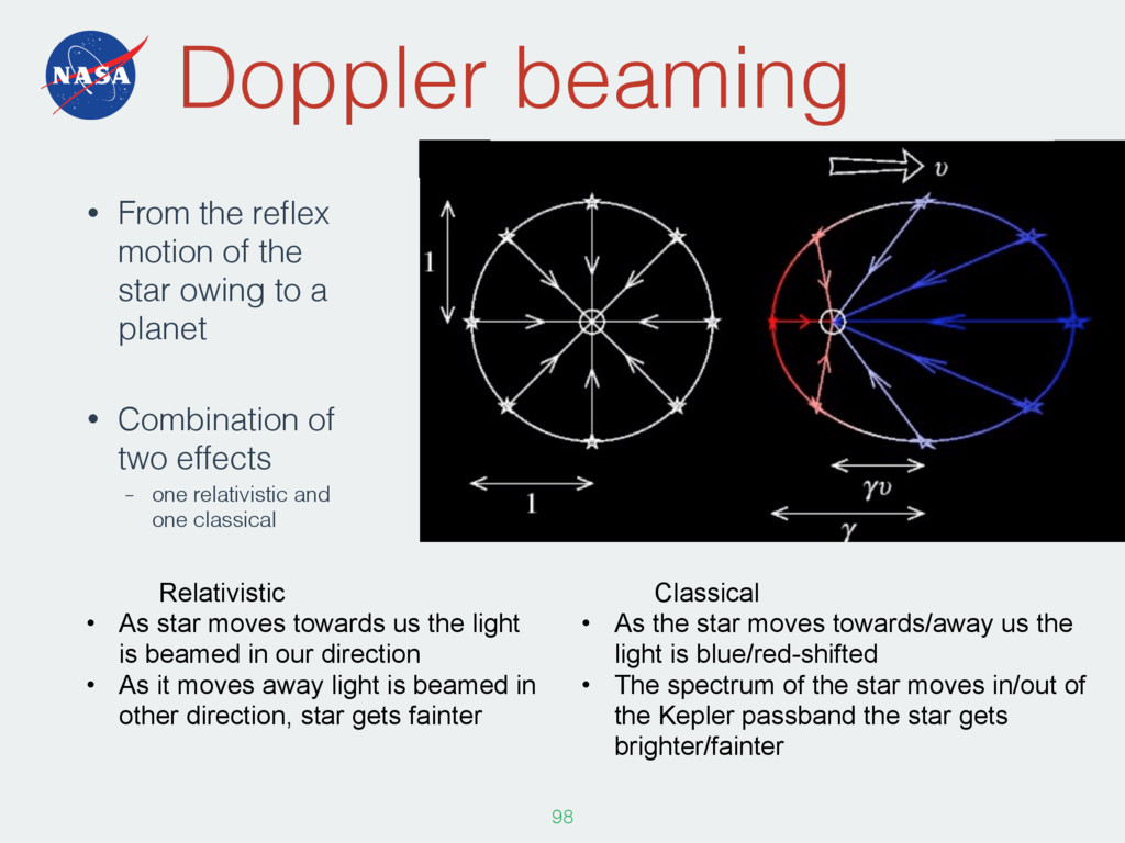
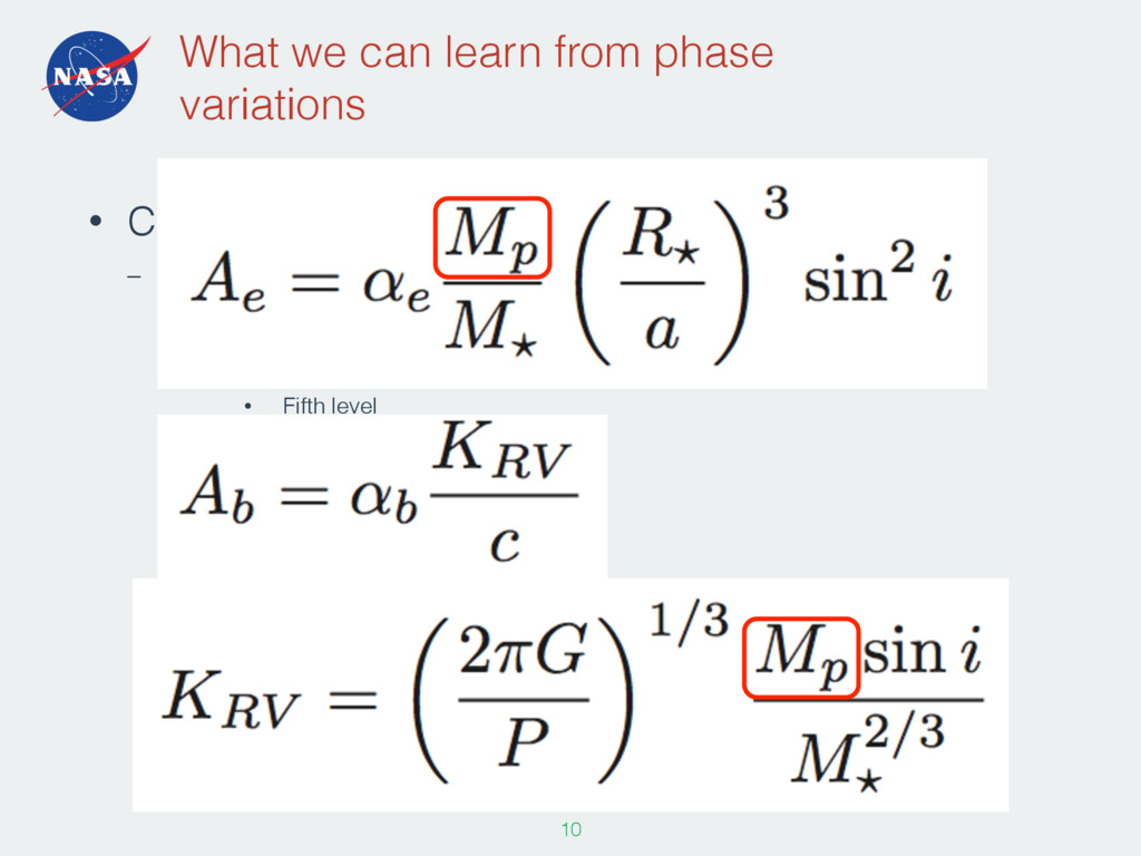
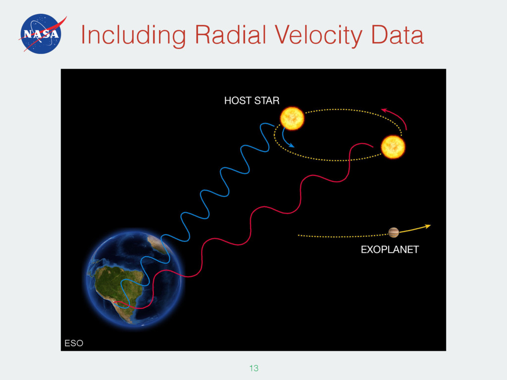
owing to a planet • Combination of two effects – one relativistic and one classical 98 Classical • As the star moves towards/away us the light is blue/red-shifted • The spectrum of the star moves in/out of the Kepler passband the star gets brighter/fainter Relativistic • As star moves towards us the light is beamed in our direction • As it moves away light is beamed in other direction, star gets fainter
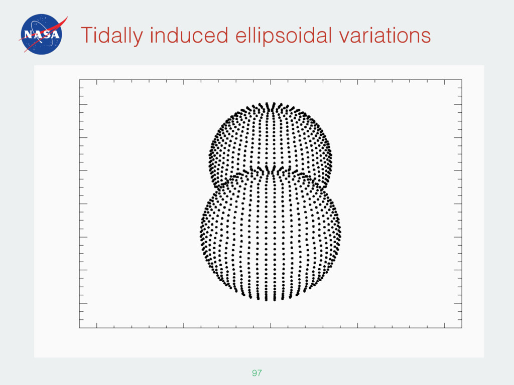
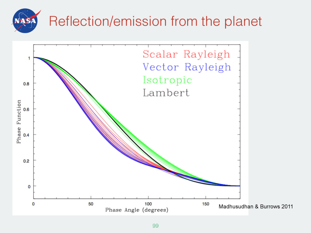
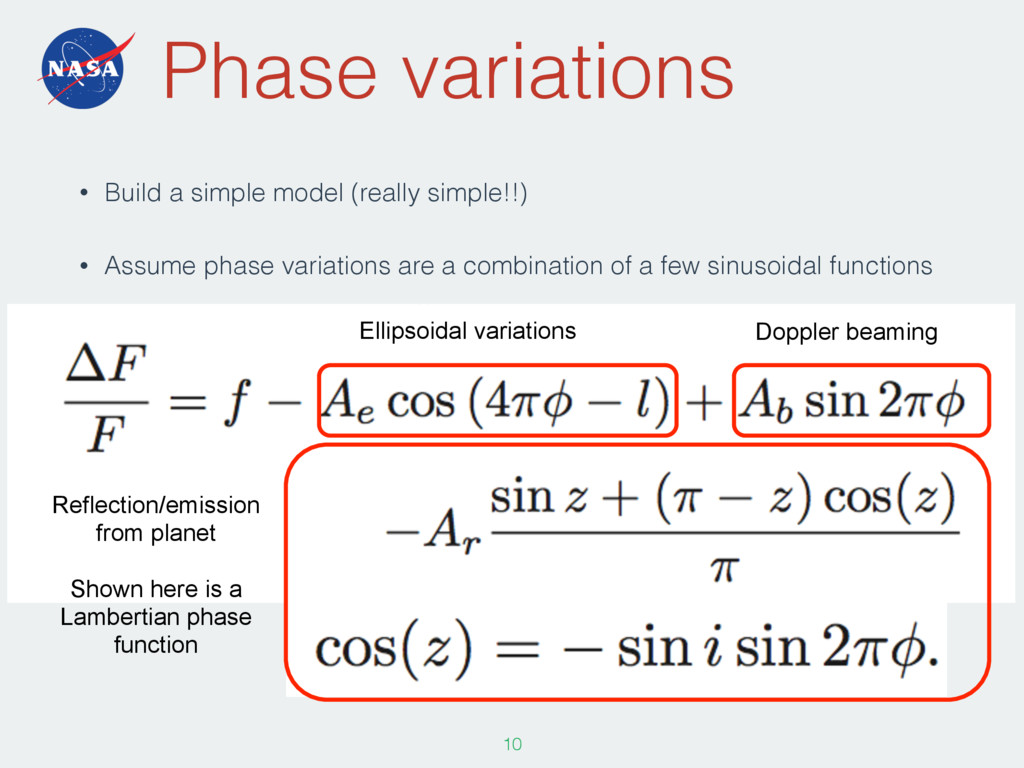
Assume phase variations are a combination of a few sinusoidal functions 100 Ellipsoidal variations Doppler beaming Reflection/emission from planet Shown here is a Lambertian phase function
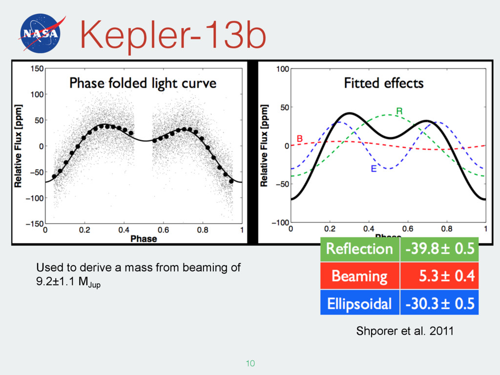
beaming and reflection from TrES-2b. • A radial velocity amplitude consistent with ground based RVs 104 Photometry Ground-based RVs Barclay et al., 2012
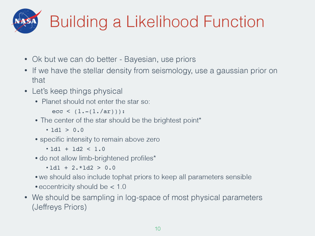
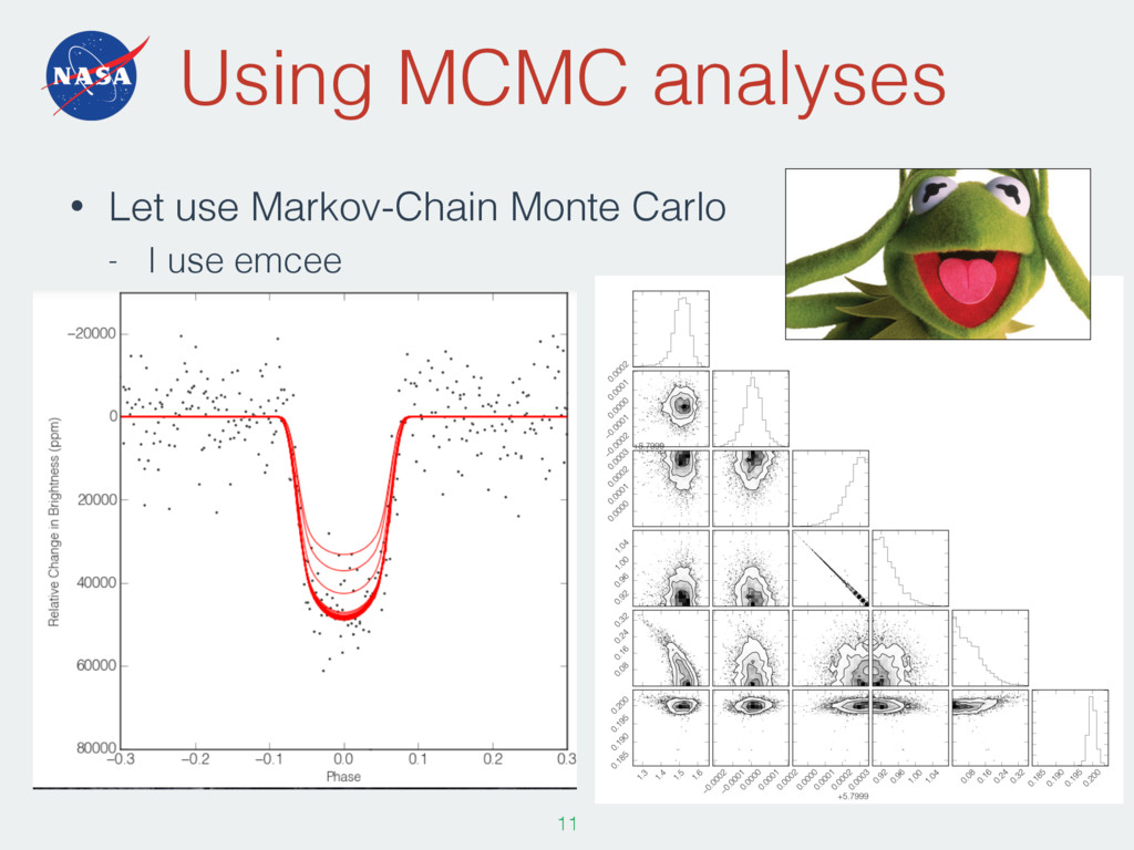
better - Bayesian, use priors • If we have the stellar density from seismology, use a gaussian prior on that • Let’s keep things physical • Planet should not enter the star so: ecc < (1.-(1./ar))): • The center of the star should be the brightest point* • ld1 > 0.0 • specific intensity to remain above zero • ld1 + ld2 < 1.0 • do not allow limb-brightened profiles* • ld1 + 2.*ld2 > 0.0 • we should also include tophat priors to keep all parameters sensible • eccentricity should be < 1.0 • We should be sampling in log-space of most physical parameters (Jeffreys Priors) 107
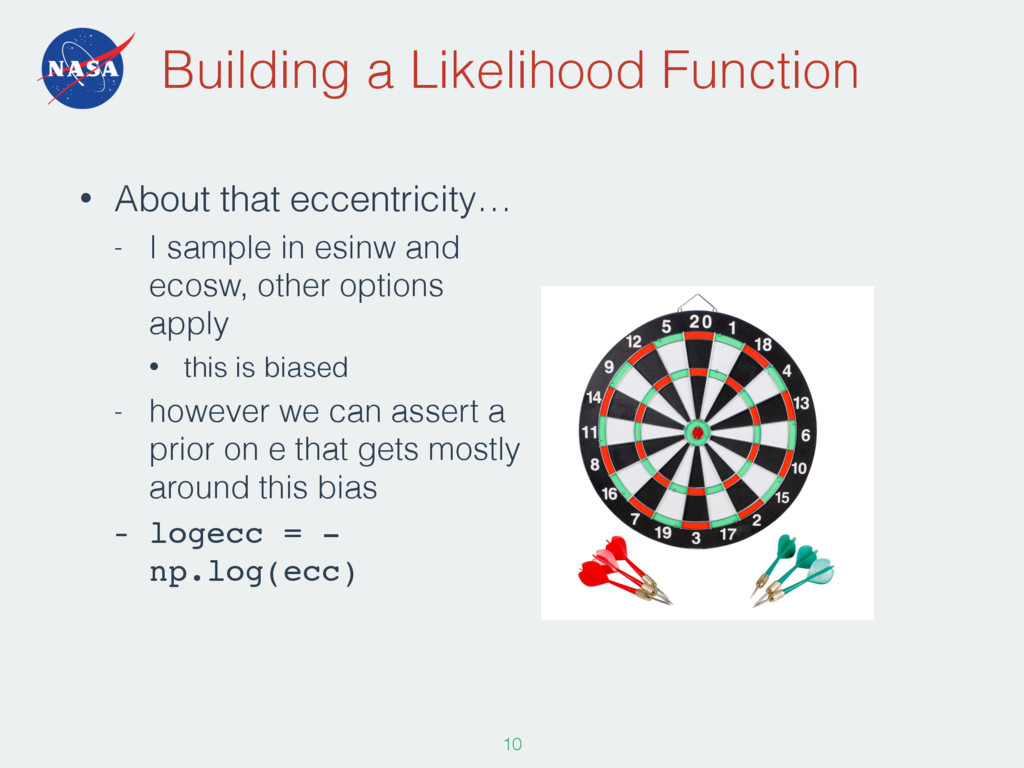
sample in esinw and ecosw, other options apply • this is biased - however we can assert a prior on e that gets mostly around this bias - logecc = - np.log(ecc) 108
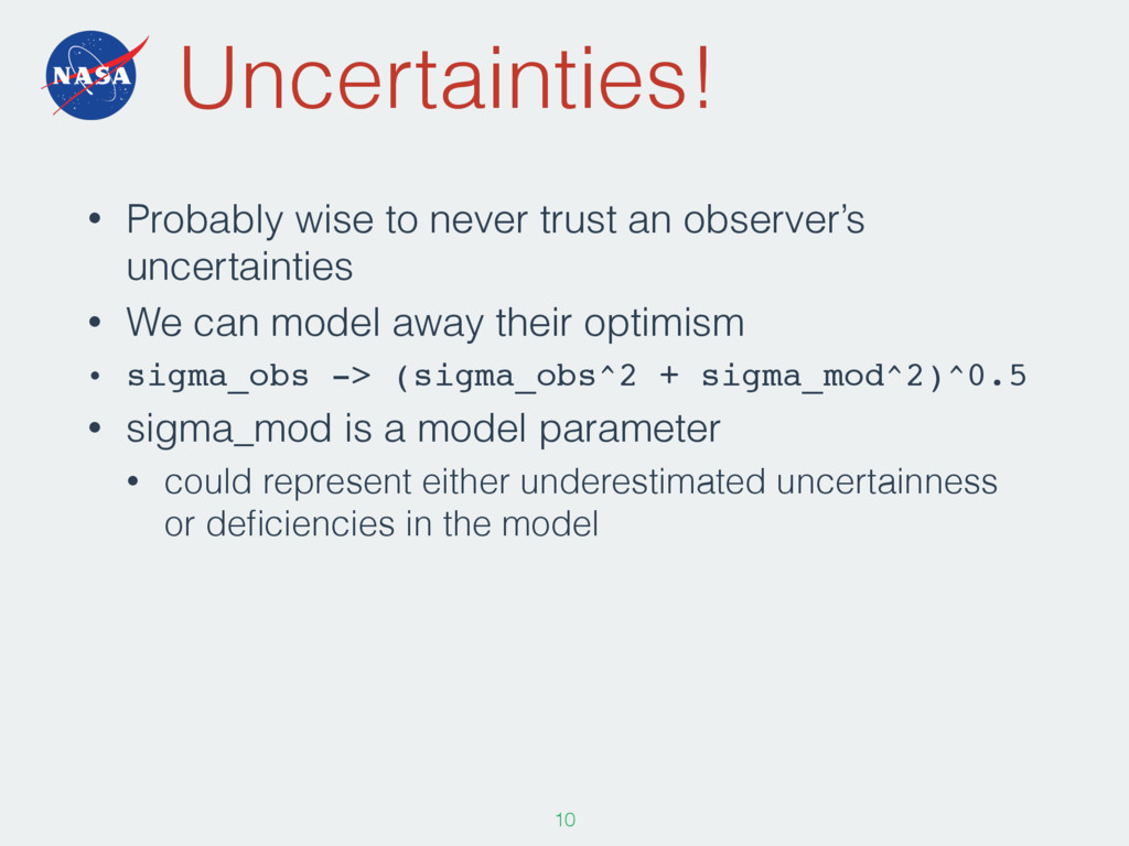
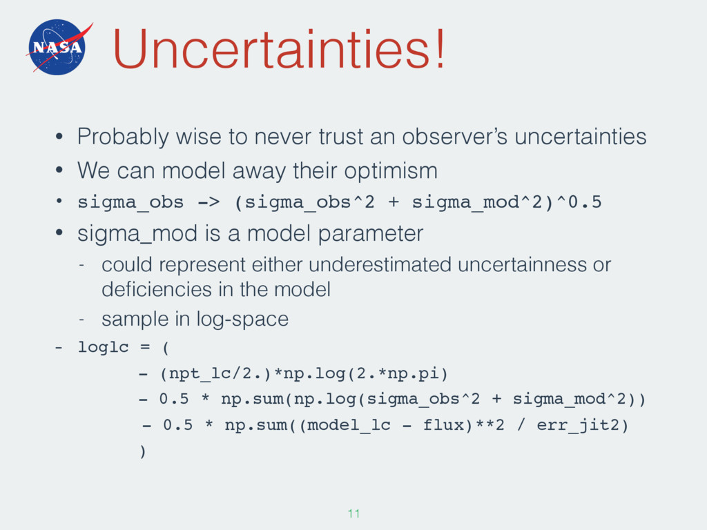
• We can model away their optimism • sigma_obs -> (sigma_obs^2 + sigma_mod^2)^0.5 • sigma_mod is a model parameter • could represent either underestimated uncertainness or deficiencies in the model 109
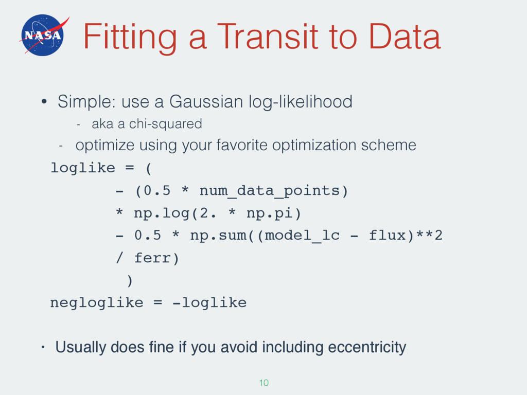
• We can model away their optimism • sigma_obs -> (sigma_obs^2 + sigma_mod^2)^0.5 • sigma_mod is a model parameter - could represent either underestimated uncertainness or deficiencies in the model - sample in log-space - loglc = ( - (npt_lc/2.)*np.log(2.*np.pi) - 0.5 * np.sum(np.log(sigma_obs^2 + sigma_mod^2)) - 0.5 * np.sum((model_lc - flux)**2 / err_jit2) ) 110
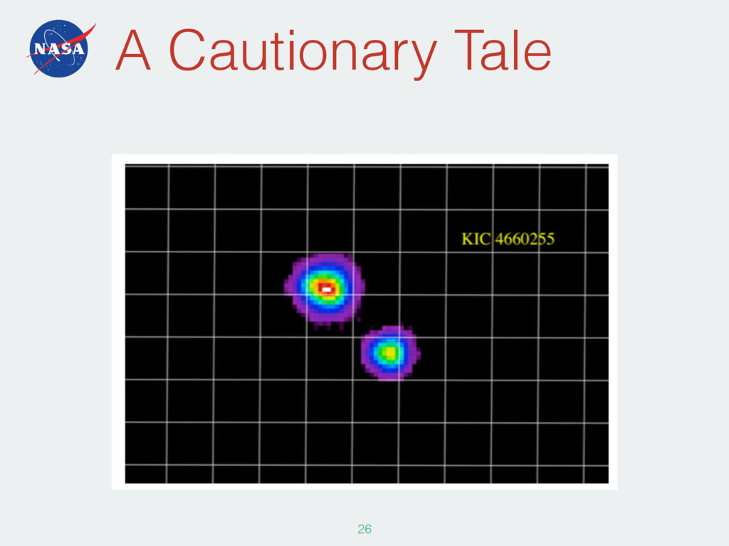
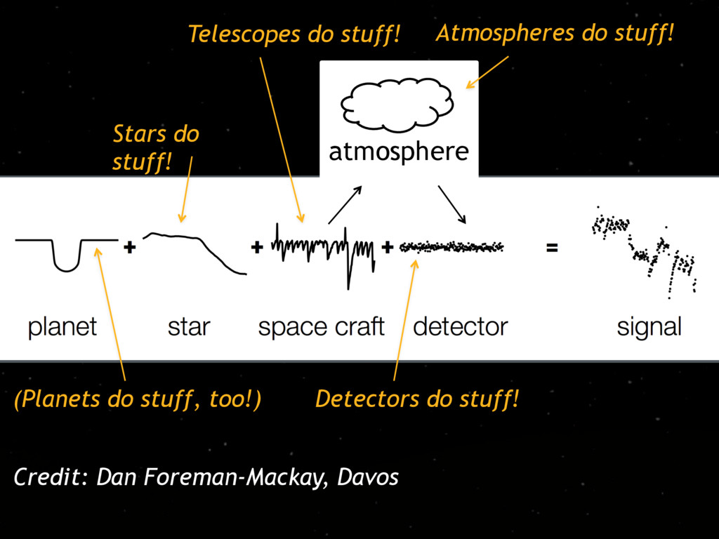
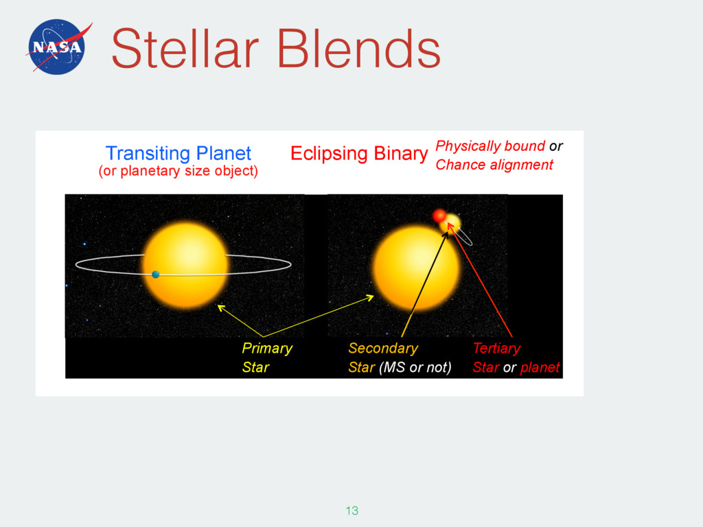
or Chance alignment Primary Star Secondary Star (MS or not) Tertiary Star or planet An observed periodic transit signal could be due to: Transiting Planet (or planetary size object)
![Gaussian Processes 115 [Ai-yi]T](https://files.speakerdeck.com/presentations/805a65e990a649a68959068c519c0d05/slide_114.jpg)