Time Series Model Comparison

Predicting US Consumer Expenditure using various types of time series models.

Transcript

1. Completed by: Maureen Stolberg Economic Forecasting Analysis PREDICTING U.S. CONSUMPTION
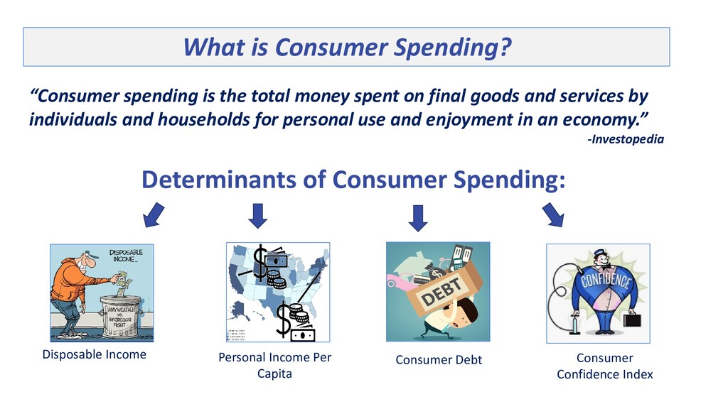
2. Determinants of Consumer Spending: Disposable Income Personal Income Per Capita Consumer Debt Consumer Confidence Index What is Consumer Spending? “Consumer spending is the total money spent on final goods and services by individuals and households for personal use and enjoyment in an economy.” -Investopedia
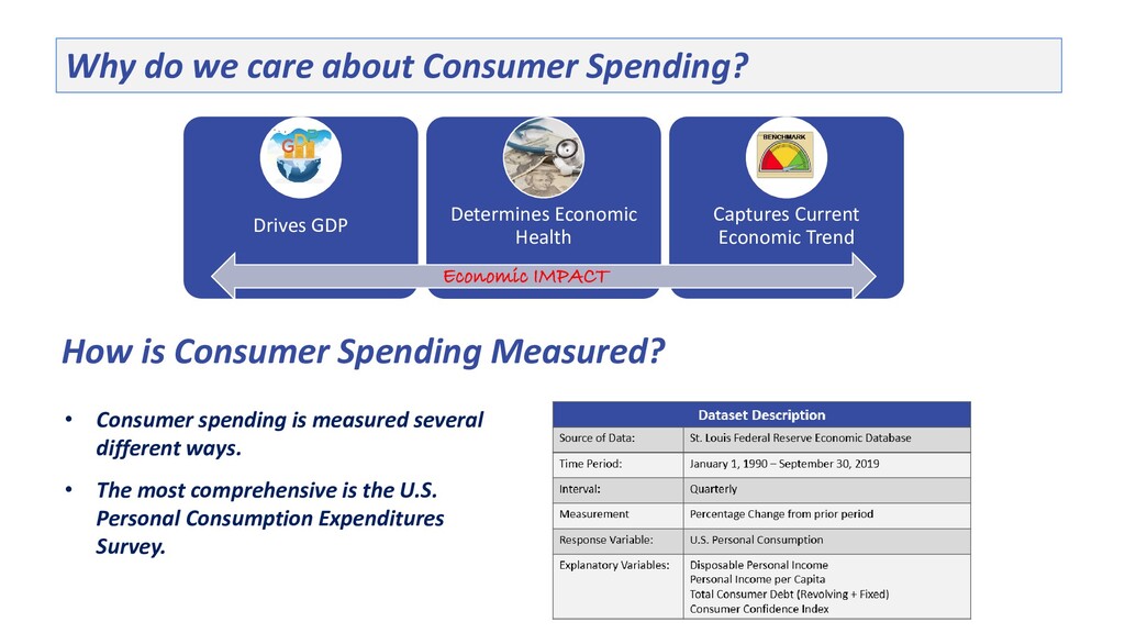
3. Why do we care about Consumer Spending? Drives GDP Determines Economic Health Captures Current Economic Trend Economic IMPACT • Consumer spending is measured several different ways. • The most comprehensive is the U.S. Personal Consumption Expenditures Survey. How is Consumer Spending Measured?
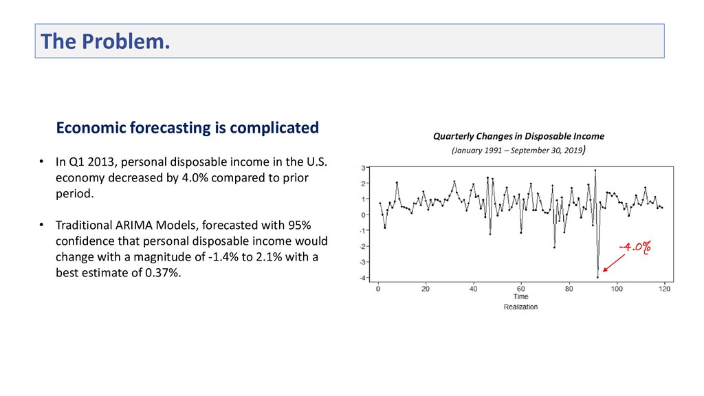
4. The Problem. -4.0% Quarterly Changes in Disposable Income (January 1991 – September 30, 2019) • In Q1 2013, personal disposable income in the U.S. economy decreased by 4.0% compared to prior period. • Traditional ARIMA Models, forecasted with 95% confidence that personal disposable income would change with a magnitude of -1.4% to 2.1% with a best estimate of 0.37%. Economic forecasting is complicated
5. The Problem. • There are several traditional linear forecasting techniques, such as AR, MA, ARIMA, and multivariate VAR have been used to effectively forecast economic time series. • These traditional methods have been reasonable successful in precision and accuracy, despite the limitations that occur when nonlinearities are present in the data. • Newer techniques, such as deep learning neural networks have been developed to forecast time series data and are being used as nonlinear forecast models As the world gets more complicated, macroeconomic relationships will become more complex and the presence of data linearities will rise. • How will the increase in data nonlinearities impact economic forecasts? • Will the performance of traditional models be able to keep up with the new AI models? Macroeconomic time series contain nonlinearities. Small changes in a few variables make predictions almost impossibly complex.
6. The Question of Interest. • The objective of this study is to compare the performance of traditional models vs. non-traditional models during periods where data nonlinearities are likely to be present. Quarterly Changes in US Consumption (January 1991 – September 30, 2019) • Key Economic decisions make by policymakers in 2017 increased the presence of data nonlinearities and created significant risks for the 2018 & 2019 economic forecasts. • As a result, many industry experts failed to accurately measure the impact of these risks and therefore consequently produced muted results. • This study will examine the ARIMA, VAR, and NNP models and compare forecasts over the same period in attempt to identify which model is more effective at picking up on the change in behavior.
7. Important Note. • Please note that in my previous video covered many of the basics, such as Stationarity vs. Non-Stationarity , the importance of differencing the data, and definition of US Consumption. • Due to restrictions on time, I will refrain from covering those topics and ask that if you are interested in learning more about the basics to please preview my last video before proceeding any further. Thanks!
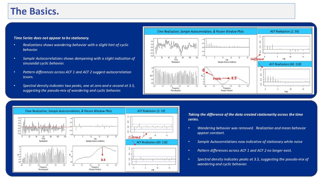
8. Time Series does not appear to be stationary. • Realizations shows wandering behavior with a slight hint of cyclic behavior. • Sample Autocorrelations shows dampening with a slight indication of sinusoidal cyclic behavior. • Pattern differences across ACF 1 and ACF 2 suggest autocorrelation issues. • Spectral density indicates two peaks, one at zero and a second at 3.5, suggesting the pseudo-mix of wandering and cyclic behavior. Peak 3.5 0 Taking the difference of the data created stationarity across the time series. • Wandering behavior was removed. Realization and mean behavior appear constant. • Sample Autocorrelations now indicative of stationary white noise • Pattern differences across ACF 1 and ACF 2 no longer exist. • Spectral density indicates peaks at 3.5, suggesting the pseudo-mix of wandering and cyclic behavior. The Basics.
9. Model Forecast Model Vs. Real Data Comparisons Model Forecast Model Vs. Real Data Comparisons VS ARIMA Models. ASE SCORES Var 1 Model VAR 2 Model 0.1119 0.1162
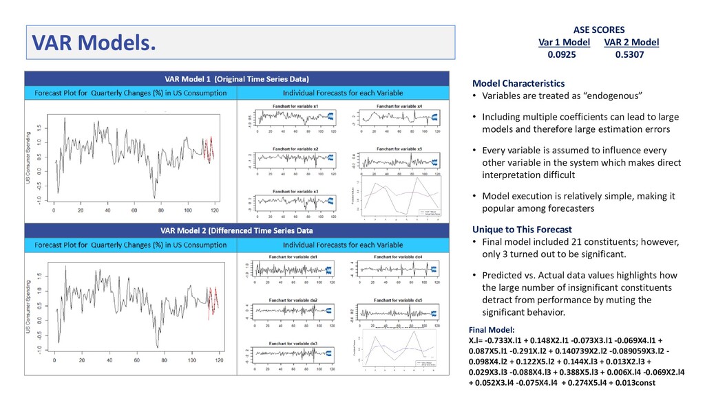
10. ASE SCORES Var 1 Model VAR 2 Model 0.0925 0.5307 VAR Models. Model Characteristics • Variables are treated as “endogenous” • Including multiple coefficients can lead to large models and therefore large estimation errors • Every variable is assumed to influence every other variable in the system which makes direct interpretation difficult • Model execution is relatively simple, making it popular among forecasters Unique to This Forecast • Final model included 21 constituents; however, only 3 turned out to be significant. • Predicted vs. Actual data values highlights how the large number of insignificant constituents detract from performance by muting the significant behavior. Final Model: X.l= -0.733X.l1 + 0.148X2.l1 -0.073X3.l1 -0.069X4.l1 + 0.087X5.l1 -0.291X.l2 + 0.140739X2.l2 -0.089059X3.l2 - 0.098X4.l2 + 0.122X5.l2 + 0.144X.l3 + 0.013X2.l3 + 0.029X3.l3 -0.088X4.l3 + 0.388X5.l3 + 0.006X.l4 -0.069X2.l4 + 0.052X3.l4 -0.075X4.l4 + 0.274X5.l4 + 0.013const
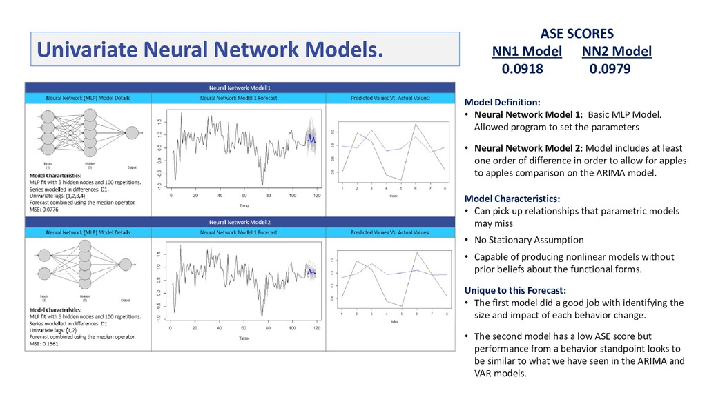
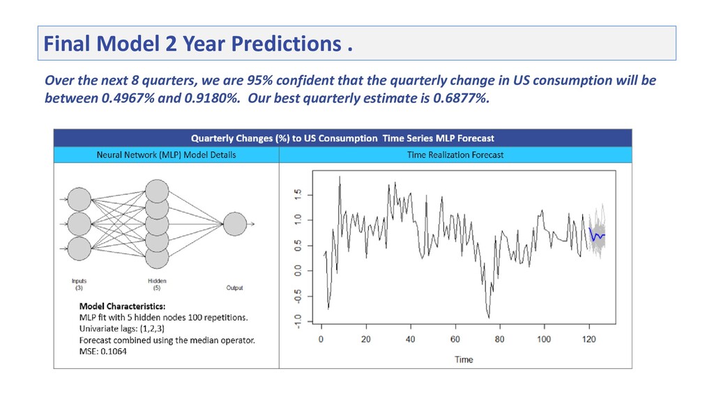
11. ASE SCORES NN1 Model NN2 Model 0.0918 0.0979 Univariate Neural Network Models. Model Definition: • Neural Network Model 1: Basic MLP Model. Allowed program to set the parameters • Neural Network Model 2: Model includes at least one order of difference in order to allow for apples to apples comparison on the ARIMA model. Model Characteristics: • Can pick up relationships that parametric models may miss • No Stationary Assumption • Capable of producing nonlinear models without prior beliefs about the functional forms. Unique to this Forecast: • The first model did a good job with identifying the size and impact of each behavior change. • The second model has a low ASE score but performance from a behavior standpoint looks to be similar to what we have seen in the ARIMA and VAR models.
12. ASE SCORES NN3 Model NN4 Model 0.1281 0.1315 Multivariate Neural Network Models. Model Characteristics: • Can pick up relationships that parametric models may miss • No Stationary Assumption • Capable of producing nonlinear models without prior beliefs about the functional forms. Model Definition: • Neural Network Model 3: Assumes that the regressors are known ahead of time. • Neural Network Model 4: Assumes that regressors are unknown-Individual regressor forecasts are used as inputs to the final model forecast. Unique to this Forecast: • Both models did a good job with identifying the size and impact of each behavior change. • The last data point in forecast conflicting directional movement- something to be cautious about
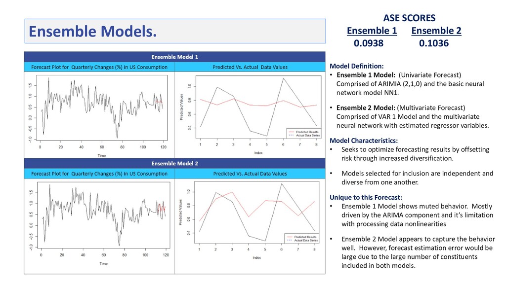
13. ASE SCORES Ensemble 1 Ensemble 2 0.0938 0.1036 Ensemble Models. Model Definition: • Ensemble 1 Model: (Univariate Forecast) Comprised of ARIMIA (2,1,0) and the basic neural network model NN1. • Ensemble 2 Model: (Multivariate Forecast) Comprised of VAR 1 Model and the multivariate neural network with estimated regressor variables. Model Characteristics: • Seeks to optimize forecasting results by offsetting risk through increased diversification. • Models selected for inclusion are independent and diverse from one another. Unique to this Forecast: • Ensemble 1 Model shows muted behavior. Mostly driven by the ARIMA component and it’s limitation with processing data nonlinearities • Ensemble 2 Model appears to capture the behavior well. However, forecast estimation error would be large due to the large number of constituents included in both models.
14. Model Comparisons.
15. Over the next 8 quarters, we are 95% confident that the quarterly change in US consumption will be between 0.4967% and 0.9180%. Our best quarterly estimate is 0.6877%. Final Model 2 Year Predictions .
16. To learn more on how the presence of neural network models is impacting the world of economic, please find some additional references below. Video Lectures: • Modeling Multivariate Time Series in Economics Harvard CMSA • Lecture 10| Recurrent Neural Networks Stanford University • Time Series Forecasting Using Recurrent Network and Vector Autoregressive Model: When and How (presented by Alliance Bernstein Chief Information Officer) Databricks Platform Additional Research References.
17. Next Steps: Future Analysis Model Types that will be examined: Univariate Analysis •ARUMA (Quarterly) Seasonal Analysis •Signal Plus Noise Model Multivariate Analysis •VAR Analysis •Neural Network •Esemble Models Thank you for Listening!!