Predicting Seasonal Influenza - Forecasting with SARIMA

Transcript

1. Predicting Seasonal Influenza Forecasting with SARIMA Maureen Stolberg, CIPM datascience@SMU For Educational Purposes Only
2. This Case Study focuses on modeling the Seasonal Flu using the ARIMA model. Data Source: World Health Organization - Flu Data Time Period: January 4, 2016 - May 31, 2020 Interval: Weekly Measurement: Number of positive flu Type A cases Important note provided by WHO regarding influenza data collected during the months of March, April, and May. The current influenza epidemiological data should be interpreted with caution as the ongoing COVID-19 pandemic might have influenced to different extents human behaviors, medical staffing procedures, as well as testing capacities at the state level. The various COVID-19 response measures to reduce SARS-CoV2 virus transmission may have an impact on influenza virus transmission within the U.S.1 * The accompanying RMarkdown file provides a detailed technical analysis. This presentation covers only the high points of the modeling. Data Reference: https://apps.who.int/flumart/Default?ReportNo=12 https://www.who.int/influenza/surveillance_monitoring/updates/latest_update_GIP_surveillance/en/ 1 For Educational Purposes Only
3. Study Objective  The Influenza Division at the Centers for Disease Control seeks to predict the traits for influenza in the U.S. which varies greatly from season to season.  Models for influenza are used for medical preparedness as well as scientific research.  For this case study, we utilized the seasonal autoregressive integrated moving average (SARIMA) model to predict the number of new influenza cases reported each week consecutively for 13 weeks (equivalent to 1 business quarter) beginning April 1, 2020. For Educational Purposes Only
4. At First Glance For Educational Purposes Only
5. First Glance at the Seasonal Data reveals important observations*. • Data clearly exhibits a seasonal pattern which peaks in January of each year with a reduction in cases during the summer months. • Total number of cases reported vary by season. However, data patterns reveal an increase in cases in each of the last two seasons. • Data is not stationary when trend and/or seasonality components are visually present in time series behavior, therefore transformations will need to be applied to make the data stationary. * Histogram (not shown here) revealed right skewed data and hence the data was log transformed before moving into the modeling phase. US National Influenza Data January 2016 – March 2020 For Educational Purposes Only
6. Data Stationarity& Transformation For Educational Purposes Only
7. The Importance of Data Stationarity A stationary time series is one whose statistical properties such as mean, variance, autocorrelation, etc. are all constant over time. • Most statistical forecasting methods are based on the assumption that the time series can be rendered stationary through the use of mathematical transformations. • Meaningful sample statistics such as means, variances, and correlations with other variables are useful as descriptors of future behavior only if the series is stationary. If the time series meets the conditions for “stationary” status and if the autocorrelations approach zero (0) as the distance between time points increases, then: A single realization can be used to estimate the following: • The mean • The variance • Autocorrelation The time series data set or “realization” must satisfy the following conditions to be considered of “Stationary” status: For Educational Purposes Only
8. The purposes of using a transformation are primarily to: • Decouple the mean and the variance so that the variability is more constant and does not depend on the mean • Enables the model to become additive and relatively simple • Confirms that the residuals, after fitting the model, are more or less normally distributed with zero mean and constant variance. This Seasonal Trend Activity chart provides us with an understanding of the structure of the variation in the data over the years, over the month, and over the entire period . Original Time Series Transformed Time Series For Educational Purposes Only
9. Zero Order Difference for Log Data Time Series: • (1-B)d factor dominates the stationary components • ACF shows a large number of positive autocorrelations out to a very high number of lags, suggesting a first difference is required. 1st Order Difference for Log Data Time Series: • Even with the first order of differencing, we observe that there is still slow residual decay in the ACF plots at a seasonal lag period. 2nd Order Difference for Log Data transformed by (1-B52): • Time series exhibits no trend or seasonality in data. • Final dataset appears stationary • Results from the Dickey Fuller (ADF) unit root test confirmed observation For Educational Purposes Only
10. Confirmation of “Data Stationarity” (Post Data Transformation) We performed a visual data review in conjunction with performing a Dicky Fuller Test* to confirm that Data is now Stationary For Educational Purposes Only • Based on the results of the Dicky Fuller Test (p-value <0.01), we were able to reject the null hypothesis that the data is non-stationary. • This falls in line with visual expectations as shown in the charts displayed below.
11. Model Identification For Educational Purposes Only
12. SARIMA Time Series Models Seasonal Autoregressive Integrated Moving Average, otherwise known as (SARIMA) is an extension of ARIMA that incorporates both non-seasonal and seasonal factors in a multiplicative model. “A SARIMA model is formed by including additional seasonal terms in the ARIMA […] The seasonal part of the model consists of terms that are very similar to the non-seasonal components of the model, but they involve backshifts of the seasonal period.” – Forecasting: Principles and Practice Seasonal Elements P: Seasonal autoregressive order. D: Seasonal difference order. Q: Seasonal moving average order. m: The # time steps for a single period. Trend Elements p: Trend autoregression order. d: Trend difference order. q: Trend moving average order. SARIMA Formula For Educational Purposes Only
13. Model Performance Evaluation Criteria Model Fit Criteria: • AIC – A measure of overall performance. • BIC – Measures overall performance but introduces a penalty for greater number of parameters to prevent overfitting. Model Performance Validation: • ASE - Most basic of methods of evaluating performance. It compares the average distance of the observed and the predicted values. • RMSE - A quadratic scoring rule that also measures the average magnitude of the error. It’s the square root of the average of squared differences between prediction and actual observation. The larger the error the greater the weight is given. The weighting also helps prevent overfitting of the model. For Educational Purposes Only
14. Parameter Estimation & Diagnostic Checking • Parameter Estimation Conditional maximum likelihood called “conditional sum of squares” was used to optimize SARIMA parameters. • Diagnostic checking. The residual correlograms (ACF and PACF), Ljung–Box Q Tests [LJUNG, BOX 1978] and Durbin– Watson test [DURBIN, WATSON 1951] were applied to test white noise (autocorrelation) of model forecasts. Whether the ACF and PACF of the residual values at various lags were settled within tolerance interval at 95% confidence limits was evaluated. For Educational Purposes Only
15. Model Identification The AIC and BIC work on the premise that the lower the score the better. The BIC system penalizes for the greater the number of parameters (overfitting). In the case of BIC, the p=0 and q=0 model is selected. The 0,0 model is not a viable for analysis. The AIC selected the p=3 and q=0 model. Ultimately, the AR(3,0), AR(2,0), and ARMA(1,1) models were selected for further analysis. P Q BIC 0 0 -2.964899 2 0 -2.958586 1 1 -2.956428 3 0 -2.953357 1 0 -2.951943 P Q AIC 3 0 -3.032584 1 2 -3.028147 2 1 -3.020932 4 0 -3.019900 3 1 -3.019788 For Educational Purposes Only
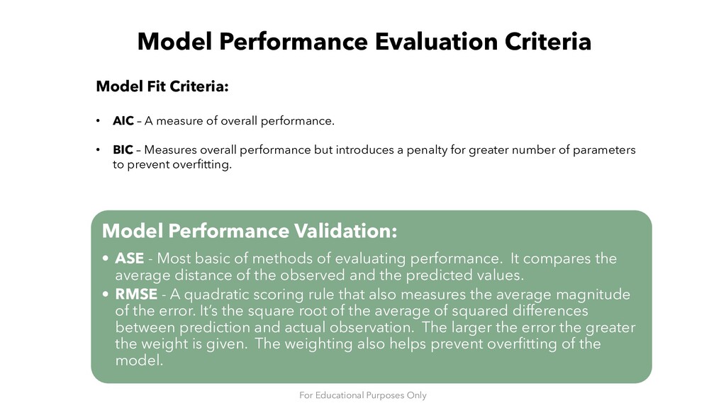
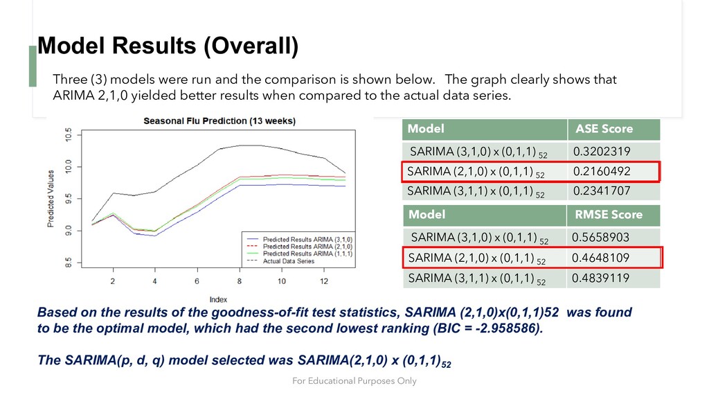
16. Model Results (Overall) Three (3) models were run and the comparison is shown below. The graph clearly shows that ARIMA 2,1,0 yielded better results when compared to the actual data series. Model ASE Score SARIMA (3,1,0) x (0,1,1) 52 0.3202319 SARIMA (2,1,0) x (0,1,1) 52 0.2160492 SARIMA (3,1,1) x (0,1,1) 52 0.2341707 Based on the results of the goodness-of-fit test statistics, SARIMA (2,1,0)x(0,1,1)52 was found to be the optimal model, which had the second lowest ranking (BIC = -2.958586). The SARIMA(p, d, q) model selected was SARIMA(2,1,0) x (0,1,1)52 Model RMSE Score SARIMA (3,1,0) x (0,1,1) 52 0.5658903 SARIMA (2,1,0) x (0,1,1) 52 0.4648109 SARIMA (3,1,1) x (0,1,1) 52 0.4839119 For Educational Purposes Only
17. Forecast – The predicted number of new influenza cases reported each week consecutively for 13 weeks beginning (Q2) April 1, 2020. Forecast Lower Upper Week 1 14758 9740 22361 Week 2 10424 5596 19418 Week 3 6802 2965 15601 Week 4 4485 1639 12270 Week 5 2604 812 8355 Week 6 1458 394 5394 Week 7 940 223 3963 Week 8 606 128 2882 Week 9 502 94 2667 Week 10 409 69 2416 Week 11 320 49 2086 Week 12 247 34 1770 Week 13 233 30 1826 For Educational Purposes Only
18. Customer Recommendations • Based on our analysis over the course of the next 13 weeks, April to June, there will be a large decrease in positive flu virus cases. • With a 95% confidence interval we estimate: • Week 0 to Week 1 a decline of 5160 positive flu cases from 19918 to 14758 (25.9%) • Week 0 to Week 13 a decline of 19685 positive flu cases from 19918 to 233 (98.8%), which is expected at this time of year. • Demand levels for medical preparedness (as it related to influenza) should start to decline during the first weeks of Q2 2020. For Educational Purposes Only