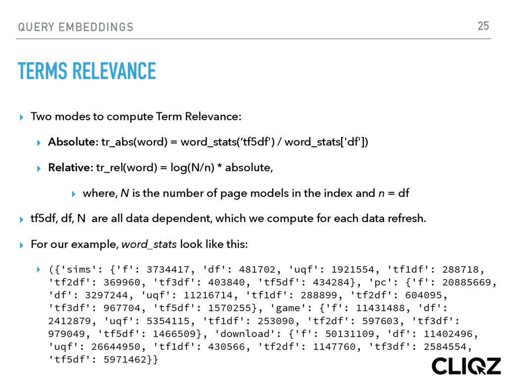
▸ Building a web scale search engine, optimized for German speaking community. ▸ Areas: Large scale Information Retrieval, Machine Learning, Deep Learning and Natural Language Processing. ▸ Mozilla Representative (2012 - Present) 2 Ankit Bahuguna (@codekee)
creating a vector model of the document [TF-IDF etc.] and searching for relevant terms of the query within the same. ▸ Aim: To give the most accurate document ranked in an order based on several parameters. 5
on matching a user query to a query in our index. ▸ Construct alternate queries and search them simultaneously. Query Similarity based on the words matched and ratio of match. ▸ Broadly, our Index: ▸ query: [<url_id1>, <url_id2>, <url_id3>, <url_id4>] ▸ url_id1 = "+0LhKNS4LViH\/WxbXOTdOQ==" {“url":"http://www.uefa.com/trainingground/skills/video/ videoid=871801.html"} 6
queries search system, two steps happen for an effective search result: ▸ RECALL: Get best candidate pages from index which closely represents query. ▸ @Cliqz: Come up with (~10k+) pages using all techniques from index (1.8+ B pages) that are most appropriate pages w.r.t query. ▸ RANKING: Rank the candidate pages based on different ranking signals. ▸ @Cliqz: Several steps. After first recall of ~10,000 pages, pre_rank prunes this list down to 100 good candidate pages. ▸ Final Ranking prunes this list of 100 to Top 3 Results. ▸ Given a user Query, find 3 good pages out of ~2 Billion Pages in Index! 7
fixed dimensional vector of floating point values. Ex. 100 dimensions ▸ Distributed Representation: Words that appear in the same contexts share semantic meaning. The meaning of the Query is defined by the floating point numbers distributed in the vector. ▸ Query Vectors are learned in an unsupervised manner. Where we focus on the context of words in sentences or queries and learn the same. For learning word representations, we employ a Neural Probabilistic Language Model (NP-LM). ▸ Similarity between queries are measured as cosine or vector distance between pair of query vectors We then get “closest queries” to a user query and fetch pages (Recall). 8 http://www.jmlr.org/papers/volume3/bengio03a/bengio03a.pdf
[ ▸ [ "2 download game pc sims”, 0.10792562365531921], ▸ [ "download full game pc sims”, 0.16451804339885712], ▸ [ "download free game pc sims”, 0.1690218299627304], ▸ [ "game pc sims the", 0.17319737374782562], ▸ [ "2 game pc sims", 0.17632317543029785], ▸ ["3 all download game on pc sims”, 0.19127938151359558] ▸ ["download pc sims the", 0.19307053089141846], ▸ ["3 download free game pc sims", 0.19705575704574585], ▸ ["2 download free game pc sims", 0.19757266342639923], ▸ ["game original pc sims", 0.1987953931093216], ▸ ["download for free game pc sims", 0.20123696327209473] ▸ ………] 9
un-supervised deep learning techniques, to learn a word representa-on C(w) which is a con-nuous vector and is both syntactically and semantically similar. ▸ More precisely, we learn a continuous representation of words and would like the distance || C(w) - C(w’) || to reflect meaningful similarity between words w and w’. ▸ vector('king') - vector('man') + vector('woman') is close to vector(‘queen') ▸ We use Word2Vec to learn word and their corresponding vectors. 10
proposes two novel model architectures for computing continuous vector representations of words from very large datasets. They are: ▸ Continuous Bag of Words (cbow) ▸ Continuous Skip Gram (skip) ▸ Word2Vec focuses on distributed representations learned by neural networks. Both models are trained using stochastic gradient descent and back propagation. 11 https://code.google.com/archive/p/word2vec/
Likelihood principle to maximize the probability of the next word wt (for "target") given the previous words h (for "history") in terms of a soft-max function: score(w_t,h) computes the compatibility of word w_t with the context h (a dot product). We train this model by maximizing its log-likelihood on the training set, i.e. by maximizing: ▸ Pros: Yields a properly normalized probabilistic model for language modeling. ▸ Cons: Very expensive, because we need to compute and normalize each probability using the score for all other V words w′ in the current context h, at every training step. 13 https://www.tensorflow.org/versions/r0.9/tutorials/word2vec/index.html
binary classification objective (logistic regression) to discriminate the real target words wt from k imaginary (noise) words w~, in the same context. ▸ For CBOW: 15 https://www.tensorflow.org/versions/r0.9/tutorials/word2vec/index.html
is to maximize: ▸ Where Q θ (D=1|w,h) is the binary logistic regression probability under the model of seeing the word w in the context h in the dataset D, calculated in terms of the learned embedding vectors θ. ▸ In practice, we approximate the expectation by drawing k contrastive words from the noise distribution. ▸ This objective is maximized when the model assigns high probabilities to the real words, and low probabilities to noise words (Negative Sampling). ▸ Performance: Way more faster. Computing loss function scales to only the number of noise words that we select “k” and not to entire Vocabulary “V”. 16 https://www.tensorflow.org/versions/r0.9/tutorials/word2vec/index.html
fox jumped over the lazy dog” ▸ Define context window size: 1. Dataset of (context, target): ▸ ([the, brown], quick), ([quick, fox], brown), ([brown, jumped], fox), ... ▸ Recall, skip-gram inverts contexts and targets, and tries to predict each context word from its target word. So, task becomes to predict 'the' and 'brown' from 'quick', 'quick' and 'fox' from 'brown', etc. Dataset of (input, output) pairs becomes: ▸ (quick, the), (quick, brown), (brown, quick), (brown, fox), ... ▸ Objective function defined over entire dataset. We optimize this with SGD using one example at a time. (or, using a mini-batch (16<=batch_size< =512)) 17 https://www.tensorflow.org/versions/r0.9/tutorials/word2vec/index.html
t, we see training case: (quick, the) ▸ Goal: Predict “the” from “quick” ▸ Next, we select “num_noise” number of noisy (contrastive) examples by drawing from some noise distribution, typically the unigram distribution, P(w). For simplicity let's say num_noise=1 and we select “sheep” as a noisy example. ▸ Next, we compute “loss” for this pair of observers and noisy examples. i.e. Objective at time step “t” becomes: ▸ Goal: Update θ (embedding parameters), to maximize this objective function. 18 https://www.tensorflow.org/versions/r0.9/tutorials/word2vec/index.html
function we obtain a gradient or derivative w.r.t embedding parameter θ. i.e. ▸ We then perform an update to the embeddings by taking a small step in the direction of the gradient. ▸ We repeat this process over the entire training set, this has the effect of 'moving' the embedding vectors around for each word until the model is successful at discriminating real words from noise words. 19 https://www.tensorflow.org/versions/r0.9/tutorials/word2vec/index.html
▸ STEP 1: Word2Vec training gives unique individual vectors for each word. [dimensionality = 100] ▸ sims: [0.01 ,0.2, ……………..…., 0.23] ▸ game : [0.21 ,0.12, ……………..…., 0.123] ▸ pc: [ -0.71 ,0.52, ……………..…., -0.253] ▸ download: [0.31 ,-0.62, ……………..…., 0.923] ▸ STEP 2: Get the term relevance for each word in the query. ▸ ‘terms_relevance’: {'sims': 0.9015615463502331, 'pc': 0.4762325748412917, 'game': 0.6077838963329699, 'download': 0.5236977938865315} 23
▸ STEP 3: Next, we calculate a centroid (or Average) of the vectors (relevance-based) for each of the words in query. This resulting vector represents our Query. Simple, Weighted Average Example: ▸ In [5]: w_vectors = [[1,1,1],[2,2,2]] ▸ In [6]: weights= [1, 0.5] ▸ In [7]: numpy.average(w_vectors, axis=0, weights=weights) ▸ array([ 1.33333333, 1.33333333, 1.33333333]) ▸ In the end, ▸ sims game pc download: [ -0.171 ,0.252, ……………..…., -0.653] {dimensionality remains 100} 24
generation for top five queries leading to all pages in our data. ▸ We collect, Top Queries for each page from PageModels ▸ ~465 Million+ Queries representing all pages in our index ▸ Learn Query Vectors for them. Size: ~700 GB on disk. ▸ How do we get similar queries: User query vs 465 Million Queries? 26
vs 465M Queries — Too Too Slow! ▸ Hashing Techniques - Not very accurate for vectors. — Vectors are semantic! ▸ The solution required: ▸ Application of cosine similarity metric. ▸ Scale to 465 million Query Vectors. ▸ Takes ~10 milli-seconds or less! ▸ Approximate Nearest Neighbor Vector Model to the rescue! 27
“Annoy” library (C++ & python wrapper) to build the Approximate nearest neighbor models. Annoy is used in production at Spotify. ▸ We can't train on all 465M queries at once, too slow. ▸ Train: 10 models or 46+ M queries each ▸ Number of Trees: 10 (explained next) ▸ Size of Models: 27 GB per shard [10 models – 270 GB+] [stored in RAM] ▸ Query all 10 shards of the cluster at runtime. Sort them based on cos. similarity. ▸ Get top 55 nearest queries to user query and fetch pages related to nearest queries. 28 https://github.com/spotify/annoy
points to any query point in sub- linear time. ▸ Build a Tree, ▸ queries in O(log n) 29 https://erikbern.com/2015/09/24/nearest-neighbor-methods-vector-models-part-1/
Tree Partitioning the Space. ▸ Nice thing : Points that are close to each other in the space are more likely to be close to each other in the tree 34 https://erikbern.com/2015/10/01/nearest-neighbors-and-vector-models-part-2-how-to-search-in-high-dimensional-spaces/
Path down the binary tree. ▸ We end up with: 7 neighbors..… Cool! 36 https://erikbern.com/2015/10/01/nearest-neighbors-and-vector-models-part-2-how-to-search-in-high-dimensional-spaces/
more than 7 neighbors? ▸ Use: Priority Queue [Traverse both sides of split - threshold based] 37 https://erikbern.com/2015/10/01/nearest-neighbors-and-vector-models-part-2-how-to-search-in-high-dimensional-spaces/
neighbors are actually outside of this leaf polygon! ▸ Use: Forest of Trees 38 https://erikbern.com/2015/10/01/nearest-neighbors-and-vector-models-part-2-how-to-search-in-high-dimensional-spaces/
a word - vector pair and Annoy stores query as integer index in its model. ▸ These mappings are stored in our key-value index “keyvi”, developed in-house @ CLIQZ, which also takes care of our entire search index. www.keyvi.org
after first fetching step from index, with higher possibility of expected page(s) being among them. ▸ The queries are now matched (in real-time) using a cosine vector similarity between query vectors as well as using classical Cliqz - IR techniques. ▸ Overall, the recall improvement from previous release is ~ 5% to 7% ▸ The translated improvement in precision-value scores is between: ~ 0.5% to 1% 40
to improve recall, which is different from conventional web search techniques. ▸ Current work: ▸ Ranking changes to include: Query/Page Similarity Metric. ▸ Query to Page Similarity using Document Vectors ▸ Improving search system for pages which are not linked to queries. ▸ And lots more …