The Neural Network House: An Environment that Adapts to its Inhabitants
Re-Delivered the paper by Michael Moser (1998) during seminar "Applications of Machine Learning in Software Engineering" for WS2015 @ Chair for Software Engineering, Technical University of Munich.
Inhabitants M. C. Mozer Proceedings of the American Association for Artificial Intelligence Spring Symposium on Intelligent Environments (pp. 110-114). Menlo Park, CA: AAAI Press. 1998 . Ankit Bahuguna M. Sc., Informatics, TU Munich [email protected] 1
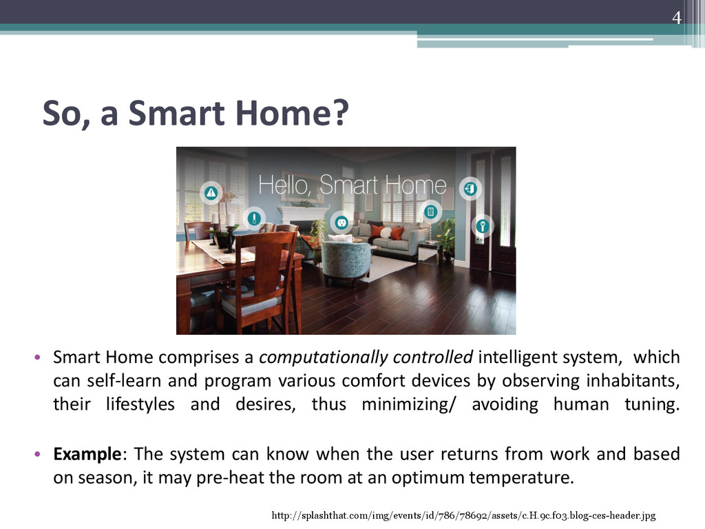
controlled intelligent system, which can self-learn and program various comfort devices by observing inhabitants, their lifestyles and desires, thus minimizing/ avoiding human tuning. • Example: The system can know when the user returns from work and based on season, it may pre-heat the room at an optimum temperature. http://splashthat.com/img/events/id/786/78692/assets/c.H.9c.f03.blog-ces-header.jpg 4
Sensors: Measure temperature, humidity, daylight or motion etc. • Controllers: PC or home automation controller. • Actuators: Motorized valves, light switches and motors etc. • Buses :Communication [wired or wireless.] • Interfaces: Human-machine or machine-to-machine interaction. 5
family. • Continuously monitoring and updating as the lifestyle changes. • Two key considerations which have to be taken care of simultaneously: ▫ Comfort of Inhabitants ▫ Energy Efficiency 6
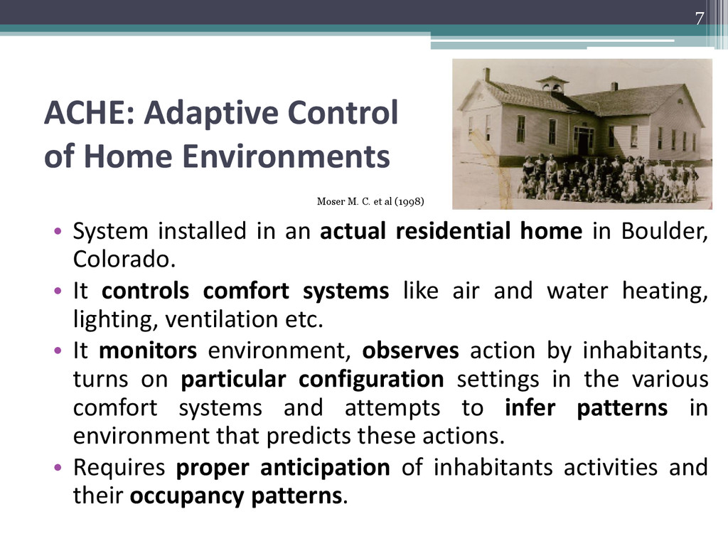
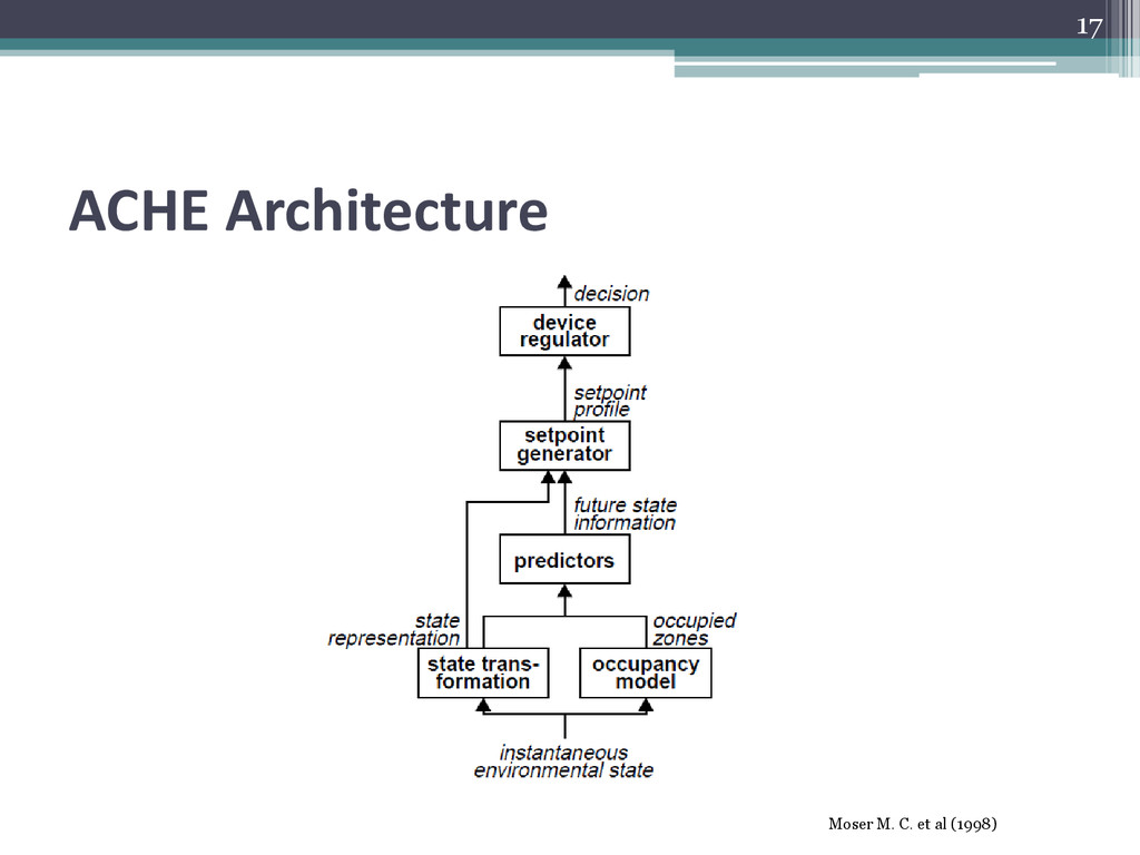
an actual residential home in Boulder, Colorado. • It controls comfort systems like air and water heating, lighting, ventilation etc. • It monitors environment, observes action by inhabitants, turns on particular configuration settings in the various comfort systems and attempts to infer patterns in environment that predicts these actions. • Requires proper anticipation of inhabitants activities and their occupancy patterns. Moser M. C. et al (1998) 7
systems in the various rooms of the home. The sensory state record: ▫ On/off status and intensity of lights; on/off status of fans and its speed; status of digital temperature etc. • System receives global information: ▫ water heating temperature; water heater energy usage; water heater outflow; furnace energy usage etc. • Also, the system has the ability to control the on/off status for actuators: intensity of light banks, ceiling fans, water heater, speakers for communication. 8
et al. [2], which created for the first time, a computational model based on mathematics and algorithms for neural networks. • In 1958, Roseblaut F. [3] put forward a pattern recognition algorithm based on a two layer computer learning algorithm. • In 1975, Paul Werbos, introduced the back propagation algorithm [4], which immediately help solved the problem of designing a circuit for the exclusive-or using just perceptron. 9
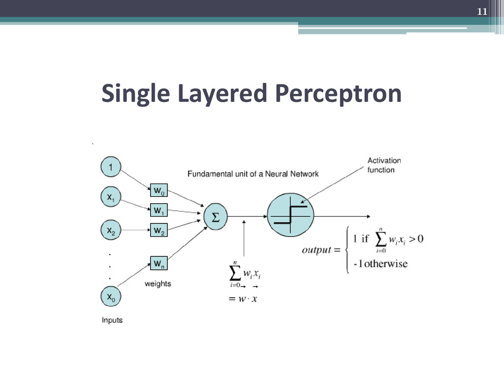
forward neural networks [5], the neurons or computation units do not form a cycle. • The network proceeds only in one direction. A perceptron is a single layered feed forward neural network, devoid of any hidden layers. • The delta rule is used in this case for training the perceptron. It calculates the errors and suggests weight adjustment based on difference in output and pre-collected sample output data. This mimics sort of gradient descent algorithm. • The output too is in form of a step function, either one value or the other. • A multilayer perceptron helps to get more continuous values as output through the use of the activation functions like logistic function: y = 1 / (1+ ex) 10
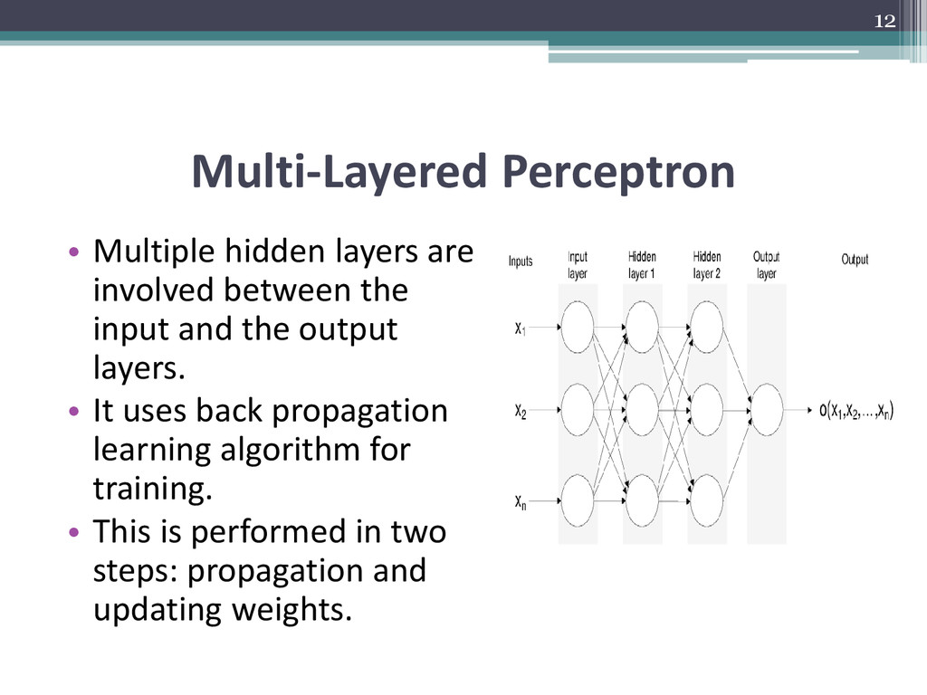
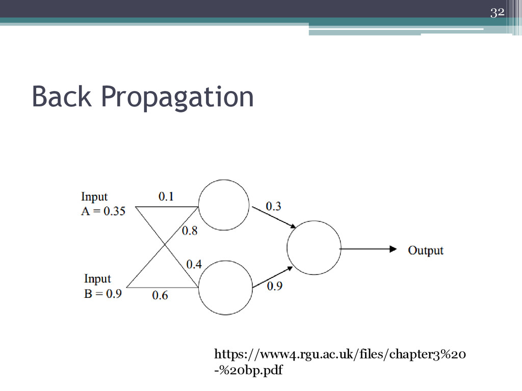
input and the output layers. • It uses back propagation learning algorithm for training. • This is performed in two steps: propagation and updating weights. 12
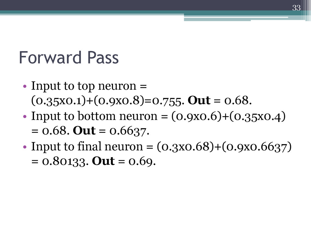
set of weights and then propagating network forward to get the output activation values. • Next we setup the backward propagation where using the sampled target values and the output activation values, we compute the deltas of all output and hidden neurons. • This information is used in the next stage of weight update, which computes the weight gradient by multiplying the output delta with input activation. At last, we subtract a ratio of this gradient from the weights and hence learn new weights. • The ratio is our learning rate which determines speed and quality of learning. This process is repeated till the network gives sufficient performance. • The back propagation algorithm tries to find such set of weights which can minimize the error (in our case the square error E) using gradient descent. • As the error needs to be minimized, this can be seen as an optimization problem. Thus, we aim to find first derivative of this error. The error is described as: • E = 1/2 (t - y)2 here, ▫ E = Squared Error; t = Training Sample’s target or expected output ▫ y = Actual computed output of the output neuron 13
to solve the problem where explicit models of user behavior is difficult to obtain. • Ex: Lighting scenario in the house. • In supervised methods, the environment is described a Markov Decision Process (MDP), with a strict need for correct input and output pairs for the learning to take place. • However, as in the lighting example, this perhaps might not be so easy to obtain in every case. Reinforcement learning tends to solve this problem, since they do not require any knowledge of MDP. 14
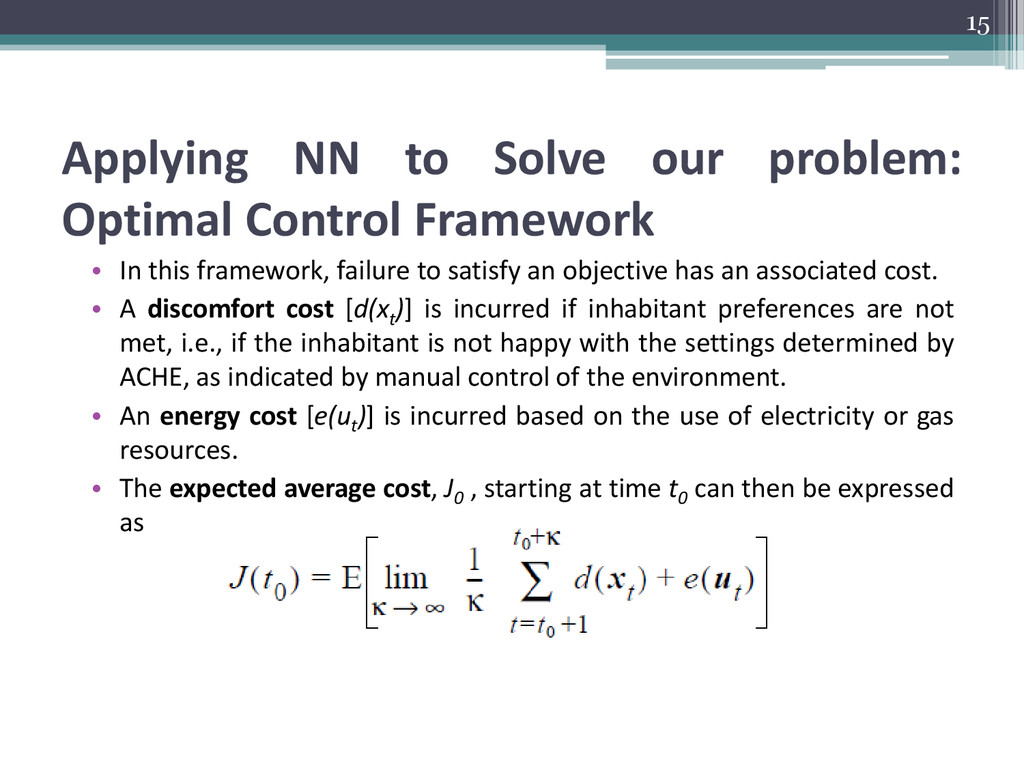
In this framework, failure to satisfy an objective has an associated cost. • A discomfort cost [d(xt )] is incurred if inhabitant preferences are not met, i.e., if the inhabitant is not happy with the settings determined by ACHE, as indicated by manual control of the environment. • An energy cost [e(ut )] is incurred based on the use of electricity or gas resources. • The expected average cost, J0 , starting at time t0 can then be expressed as 15
from state xt to decisions ut , such that J(t0 ) is minimized. • This now has become an optimization problem (viz., minimization) and we can use neural networks with back propagation to solve it. • The costs are measured in terms of same currency i.e., dollars. • Ex.: Predictive model for hot water temperature = f(current indoor temperature, outdoor temperature, status of electric water heaters, inhabitant_usage_time); • This is a simple model of the house and water heater, with neural network that learns deviations from simple model and the actual behavior of house. 16
is difficult. • The anticipation of both the environment and inhabitants behavior is not easy: non stationary and stochastic in nature. • Devices behave non linearly. Finding a set point profile is difficult. • Multiple interacting devices are required to be controlled simultaneously and optimally keeping in mind both energy consumption and comfort of inhabitants. 19
Caters two most important objectives: comfort to the inhabitants and energy conservation. • System uses both unsupervised and reinforcement learning techniques. It is flexible, thus can switch it’s method of learning to get accurate results. • Neural networks take less formal statistical training to develop. • They can implicitly detect complex non-linear relationship between independent and dependent variables. 20
patterns? • System fails to take into consideration the irregularities which occur in lives of the individuals. • System has a policy of testing its optimal settings in favor of conserving energy, where many a times, lower value than the pre-set comfort value is suggested, this may cause some discomfort. • Neural networks are often accused of being prone to over-fitting. 21
in any general purpose house. • The seminal work was published 17 years ago. Since then, a number of emerging technologies and platforms have caused a revolution in this area • Ex: wireless sensor networks, internet and cloud based computing, emergence of mobile computing platform, reduction in the cost of computational devices, etc. 22
thermostats and house hold devices which are programmable using your smartphone. • Data collected over time can be saved in the cloud and cross analyzed with respect to the other inhabitants in the same area of residence, for better predictions. • Google bought Nest for $3.2 Billion; Samsung acquired SmartThings for $200 Million. • Smart Homes are way more real now! 23
that adapts to it’s Inhabitants, Proceedings of the American Association for Artificial Intelligence Spring Symposium on Intelligent Environments (pp. 110- 114). Menlo Park, CA: AAAI Press, 1998. 2. McCulloch, Warren; Walter Pitts, A Logical Calculus of Ideas Immanent in Nervous Activity, Bulletin of Mathematical Biophysics 5 (4): 115133.doi:10.1007/BF02478259, 1943. 3. Rosenblatt, F., The Perceptron: A Probabilistic Model For Information Storage And Organization In The Brain, Psychological Review 65 (6): 386408. doi:10.1037/h0042519. PMID 13602029, 1958. 4. Werbos, P.J., Beyond Regression: New Tools for Prediction and Analysis in the Behavioral Sciences, 1975. 5. Christopher M. Bishop, Pattern Recognition and Machine Learning (Information Science and Statistics), Page 227- Springer, 2007 24
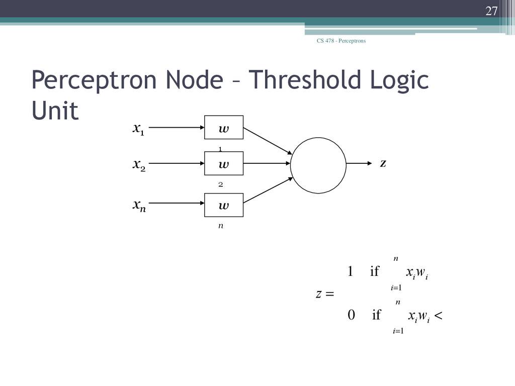
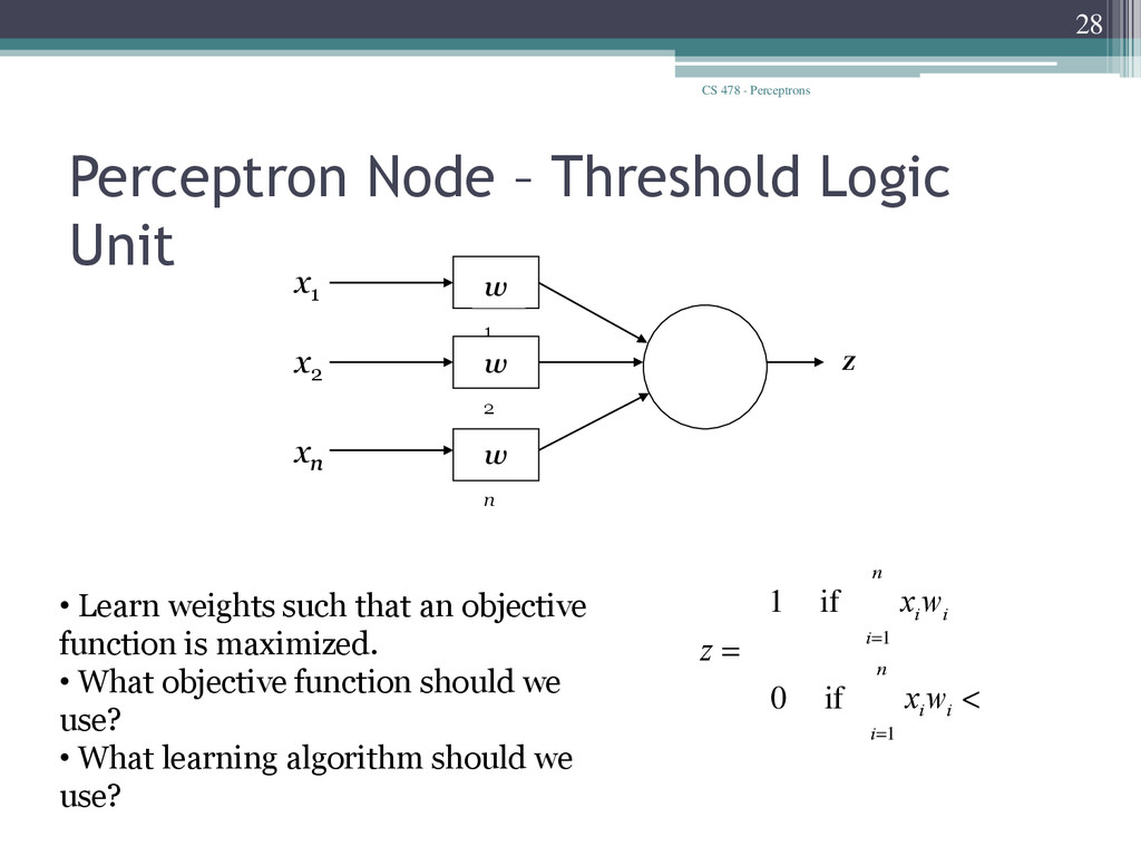
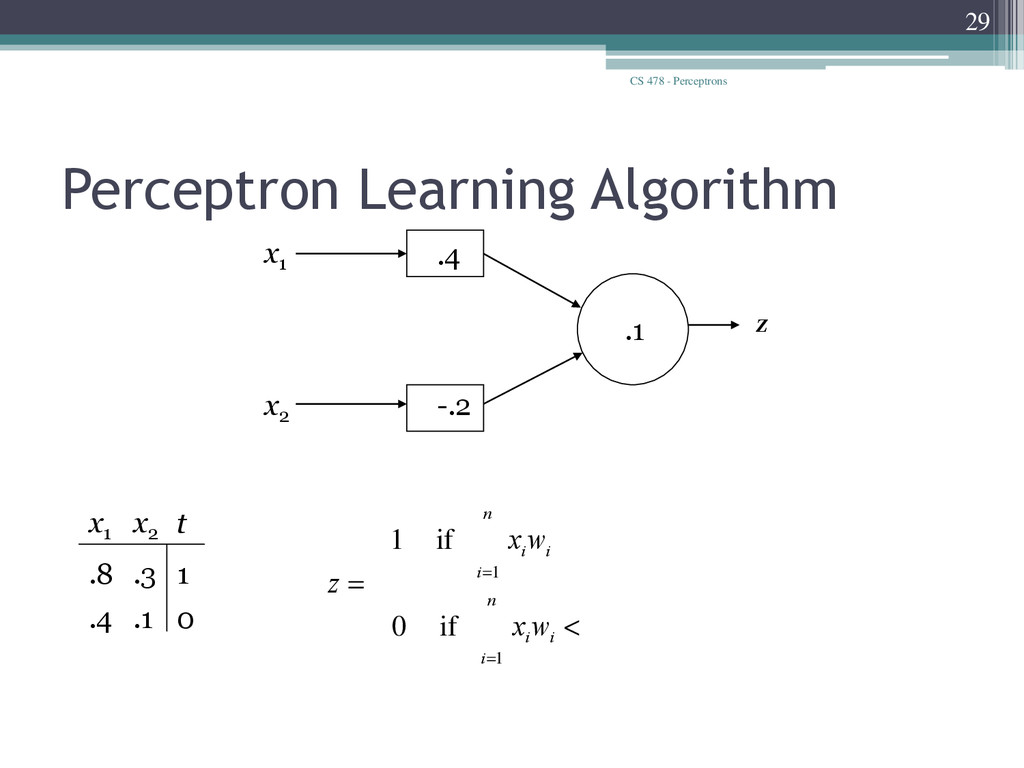
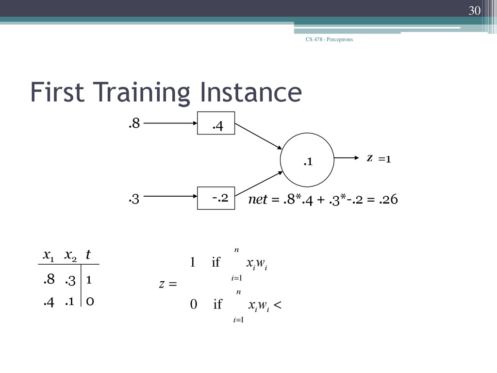
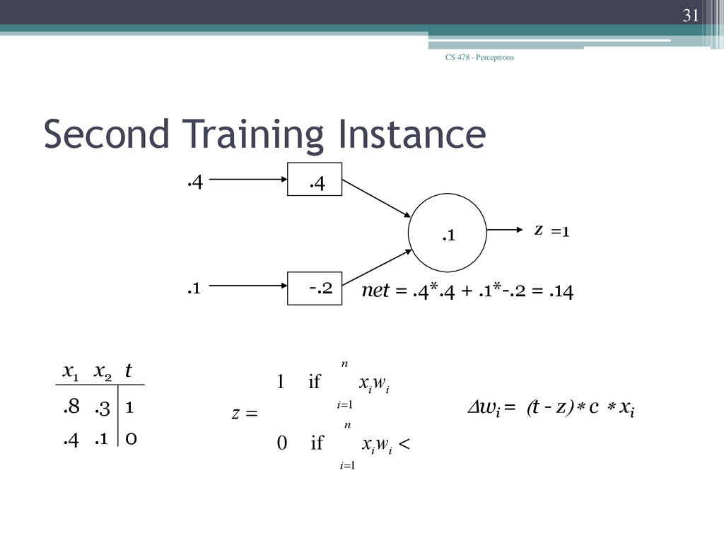
Unit x1 xn x2 w 1 w 2 w n z q q q < = ³ å å = = i n i i i n i i w x z w x 1 1 if 0 if 1 • Learn weights such that an objective function is maximized. • What objective function should we use? • What learning algorithm should we use?
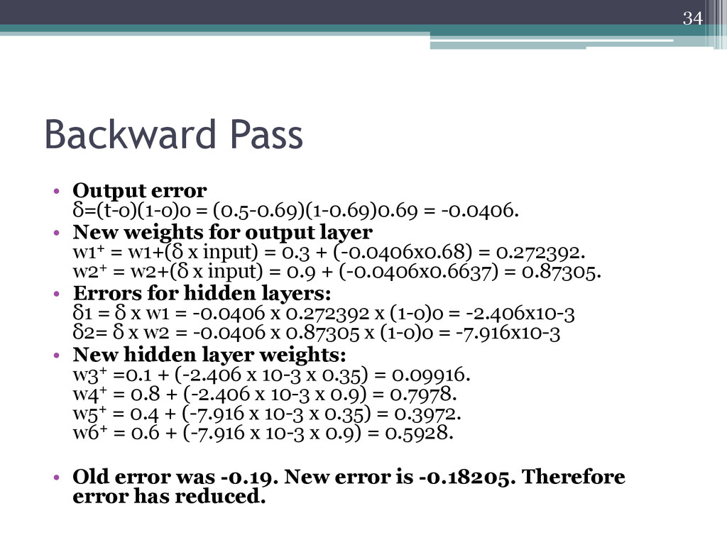
• New weights for output layer w1+ = w1+(δ x input) = 0.3 + (-0.0406x0.68) = 0.272392. w2+ = w2+(δ x input) = 0.9 + (-0.0406x0.6637) = 0.87305. • Errors for hidden layers: δ1 = δ x w1 = -0.0406 x 0.272392 x (1-o)o = -2.406x10⁻³ δ2= δ x w2 = -0.0406 x 0.87305 x (1-o)o = -7.916x10⁻³ • New hidden layer weights: w3+ =0.1 + (-2.406 x 10-3 x 0.35) = 0.09916. w4+ = 0.8 + (-2.406 x 10-3 x 0.9) = 0.7978. w5+ = 0.4 + (-7.916 x 10-3 x 0.35) = 0.3972. w6+ = 0.6 + (-7.916 x 10-3 x 0.9) = 0.5928. • Old error was -0.19. New error is -0.18205. Therefore error has reduced. 34