SLIDES: DISCLAIMER: These slides are meant to complement the oral presentation. Use out of context at your own risk. This material is based upon work supported by the U.S. Department of Energy Office of Science, Office of Advanced Scientific Computing Research, Applied Mathematics program under Award Number DE-SC-0011077. PAUL CONSTANTINE Ben L. Fryrear Assistant Professor Applied Mathematics & Statistics Colorado School of Mines activesubspaces.org! @DrPaulynomial! Joint with: Prof. David Gleich Purdue, CS Prof. Michael Wakin School of Mines, EE Dr. Armin Eftekhari UT Austin, Math
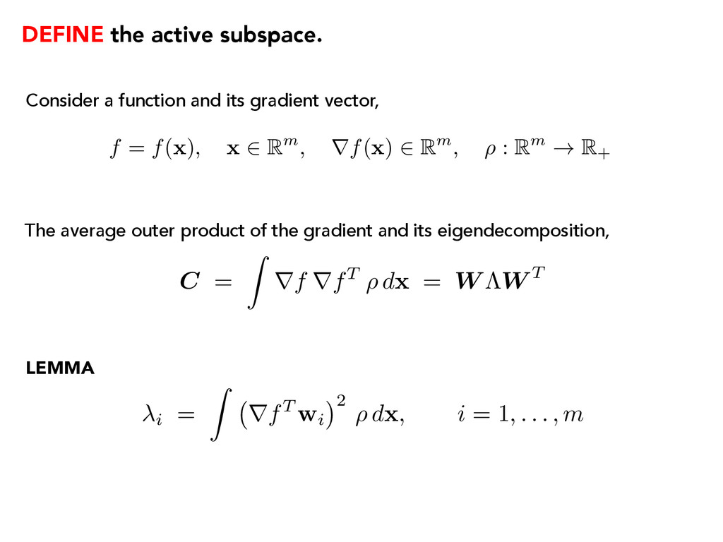
vector, The average outer product of the gradient and its eigendecomposition, f = f( x ), x 2 Rm, rf( x ) 2 Rm, ⇢ : Rm ! R + C = Z rf rfT ⇢ d x = W ⇤W T i = Z rfT wi 2 ⇢ d x , i = 1, . . . , m LEMMA
and fj = f( xj) Approximate with Monte Carlo Equivalent to SVD of samples of the gradient xj ⇠ ⇢ C ⇡ 1 N N X j=1 rfj rfT j = ˆ W ˆ ⇤ ˆ W T 1 p N ⇥ rf1 · · · rfN ⇤ = ˆ W p ˆ ⇤ ˆ V T rfj = rf( xj)
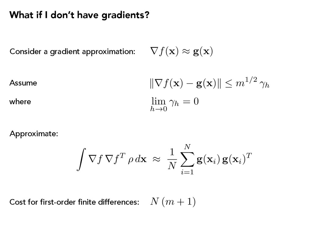
g ( x )k m1/2 h lim h!0 h = 0 rf( x ) ⇡ g ( x ) Consider a gradient approximation: where Cost for first-order finite differences: N (m + 1) Z rf rfT ⇢ d x ⇡ 1 N N X i=1 g ( xi) g ( xi)T Approximate:
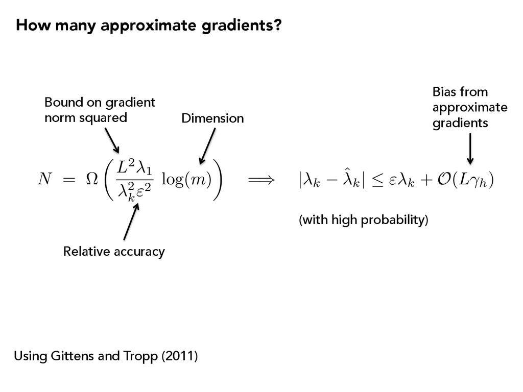
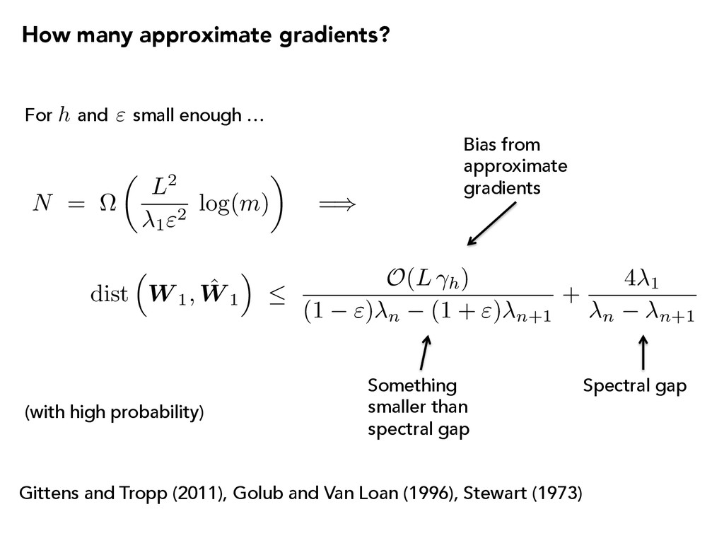
m ) ◆ = ) | k ˆk | " k + O ( L h) Using Gittens and Tropp (2011) How many approximate gradients? Bound on gradient norm squared Relative accuracy Dimension (with high probability) Bias from approximate gradients
h) (1 ") n (1 + ") n+1 + 4 1 n n+1 Gittens and Tropp (2011), Golub and Van Loan (1996), Stewart (1973) (with high probability) Spectral gap N = ⌦ ✓ L2 1"2 log( m ) ◆ = ) Something smaller than spectral gap For and small enough … " h Bias from approximate gradients How many approximate gradients?
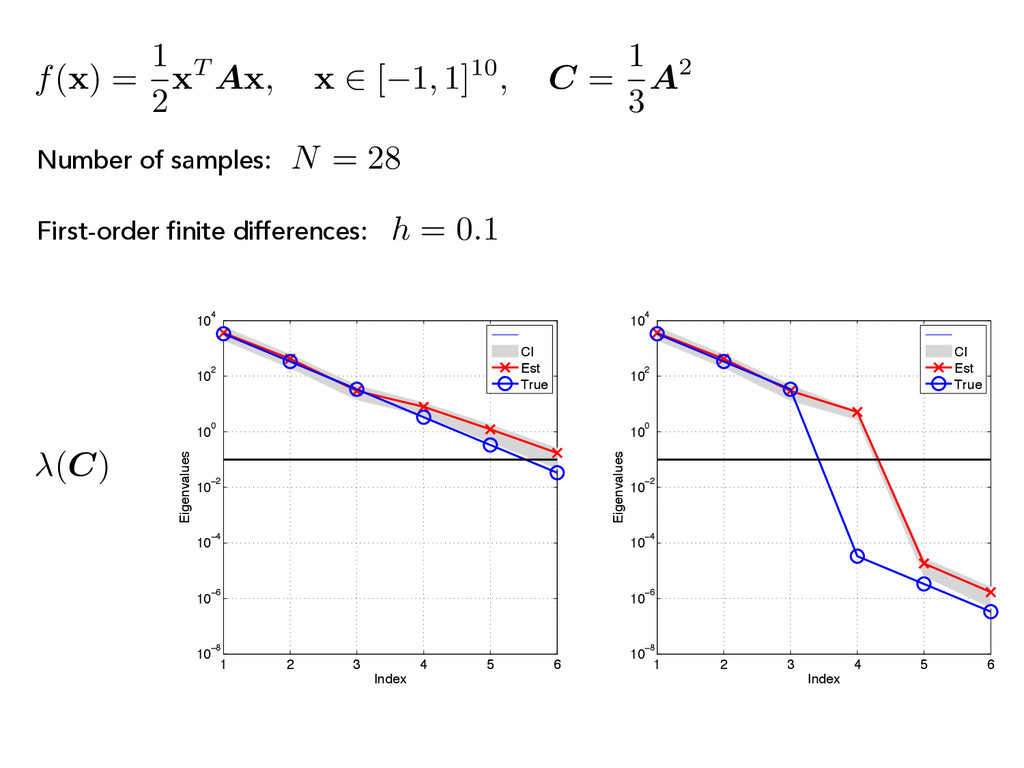
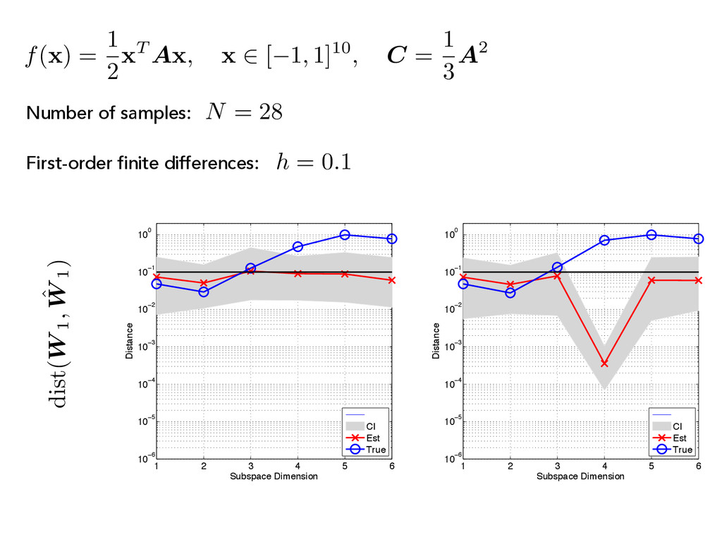
x 2 [ 1, 1]10, C = 1 3 A2 1 2 3 4 5 6 10−8 10−6 10−4 10−2 100 102 104 Index Eigenvalues CI Est True 1 2 3 4 5 6 10−8 10−6 10−4 10−2 100 102 104 Index Eigenvalues CI Est True (C) First-order finite differences: h = 0.1 N = 28 Number of samples:
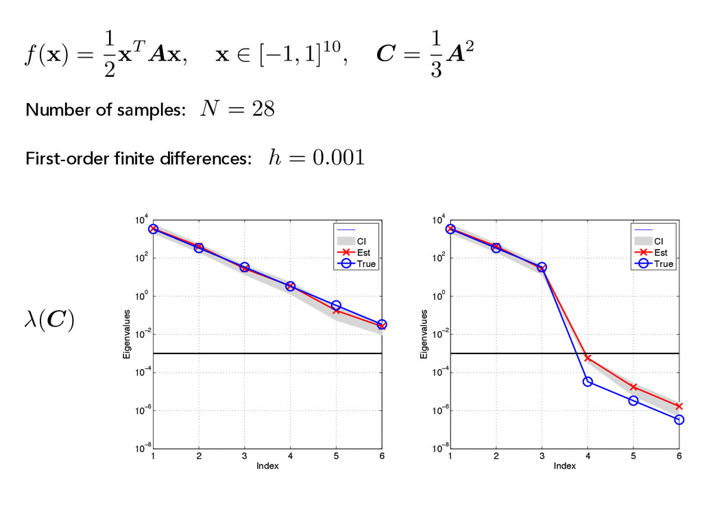
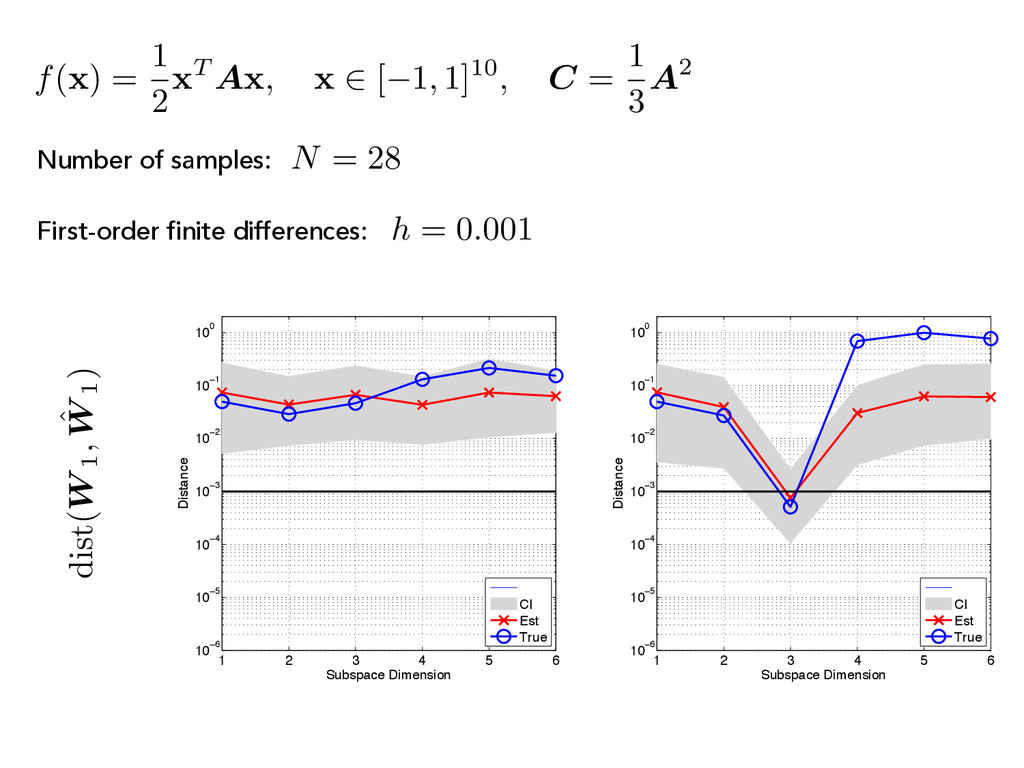
A x , x 2 [ 1, 1]10, C = 1 3 A2 (C) First-order finite differences: N = 28 Number of samples: 1 2 3 4 5 6 10−8 10−6 10−4 10−2 100 102 104 Index Eigenvalues CI Est True 1 2 3 4 5 6 10−8 10−6 10−4 10−2 100 102 104 Index Eigenvalues CI Est True
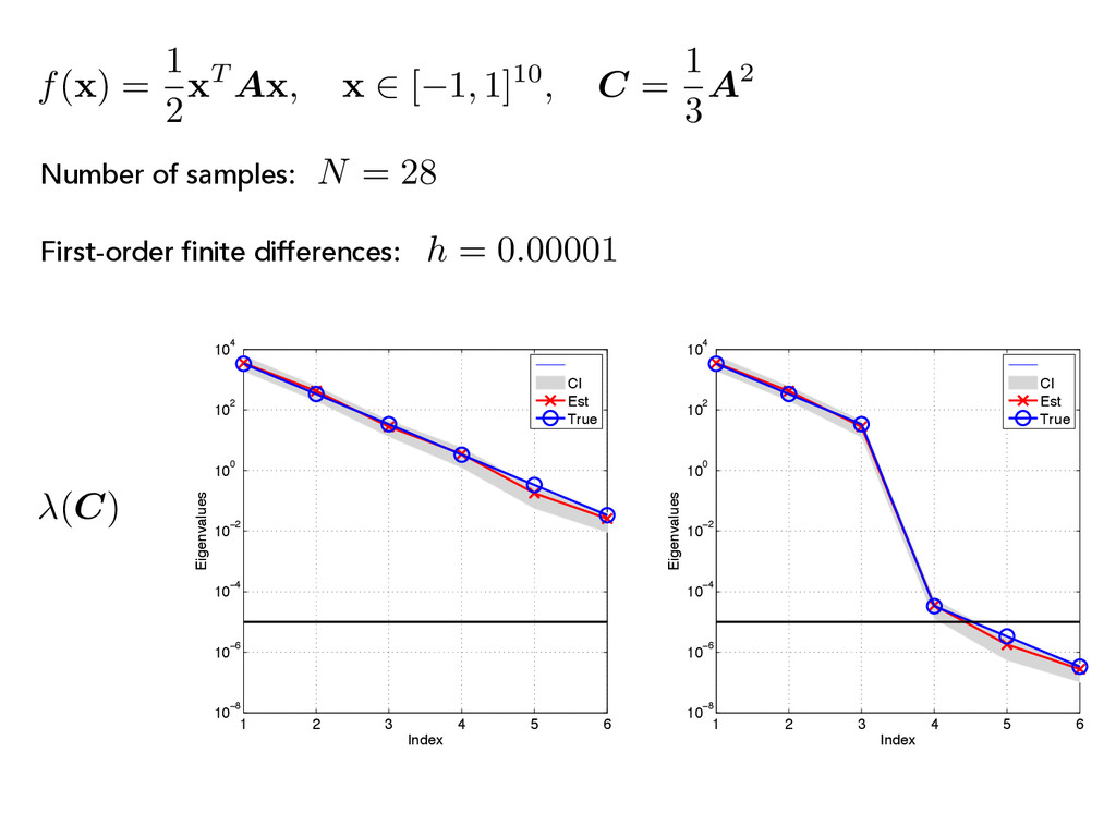
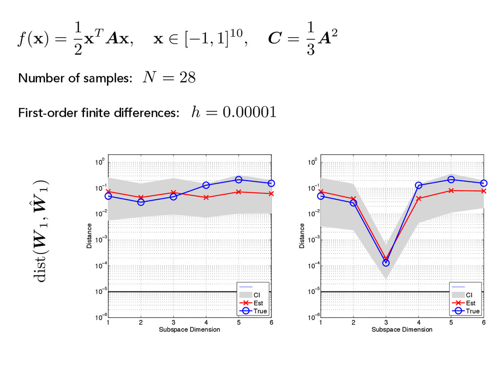
A x , x 2 [ 1, 1]10, C = 1 3 A2 (C) First-order finite differences: N = 28 Number of samples: 1 2 3 4 5 6 10−8 10−6 10−4 10−2 100 102 104 Index Eigenvalues CI Est True 1 2 3 4 5 6 10−8 10−6 10−4 10−2 100 102 104 Index Eigenvalues CI Est True
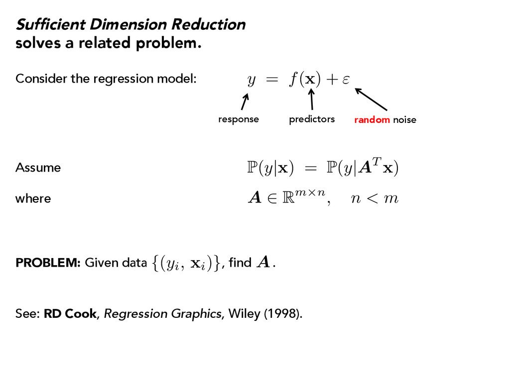
, find . y = f( x ) + " P(y| x ) = P(y|AT x ) Consider the regression model: predictors response random noise Assume where A 2 Rm⇥n, n < m {(yi, xi)} A See: RD Cook, Regression Graphics, Wiley (1998).
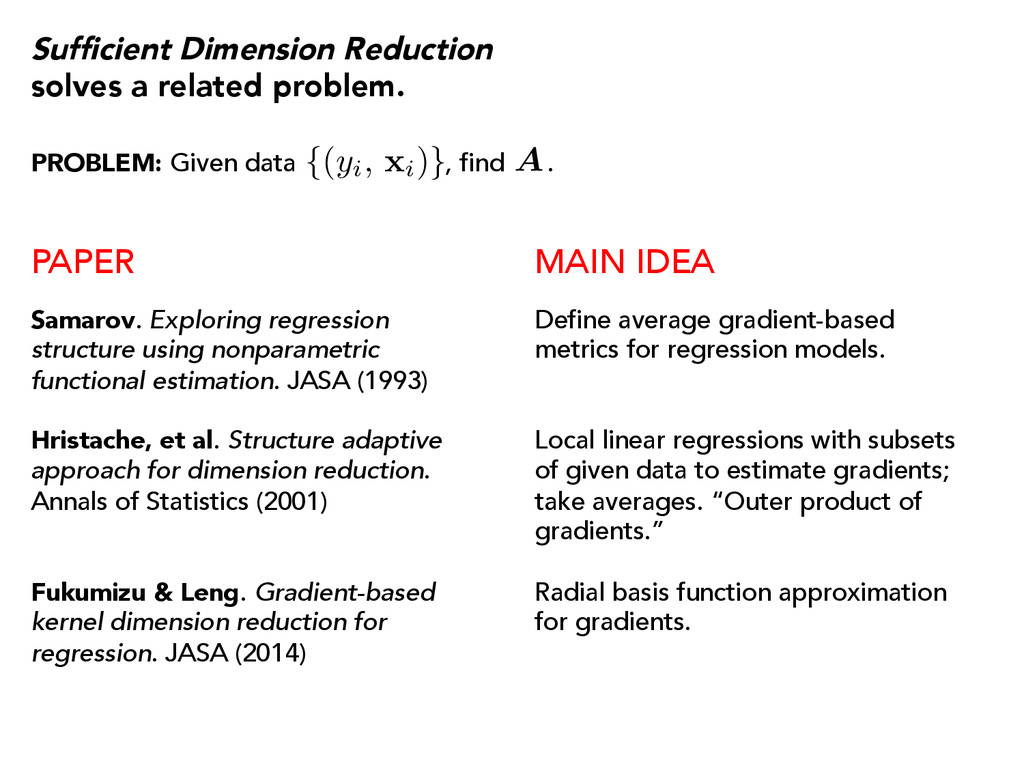
PROBLEM: Given data , find . {(yi, xi)} A Samarov. Exploring regression structure using nonparametric functional estimation. JASA (1993) Define average gradient-based metrics for regression models. Hristache, et al. Structure adaptive approach for dimension reduction. Annals of Statistics (2001) Local linear regressions with subsets of given data to estimate gradients; take averages. “Outer product of gradients.” Fukumizu & Leng. Gradient-based kernel dimension reduction for regression. JASA (2014) Radial basis function approximation for gradients.
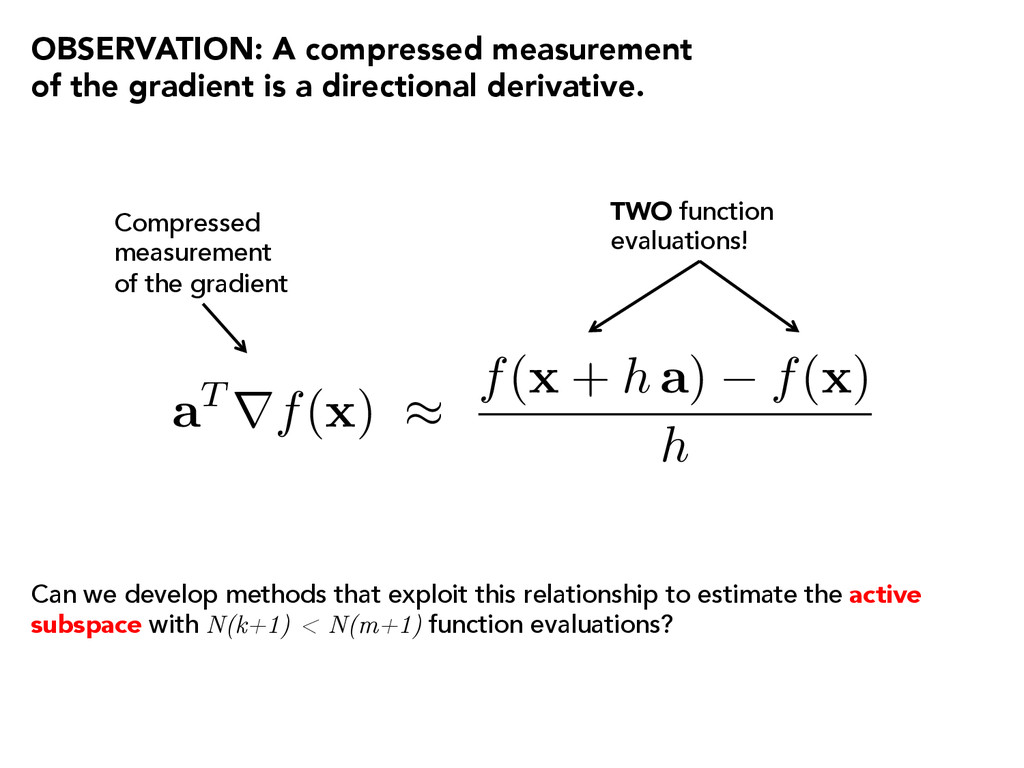
derivative. a T rf( x ) ⇡ f( x + h a ) f( x ) h Compressed measurement of the gradient TWO function evaluations! Can we develop methods that exploit this relationship to estimate the active subspace with N(k+1) < N(m+1) function evaluations?
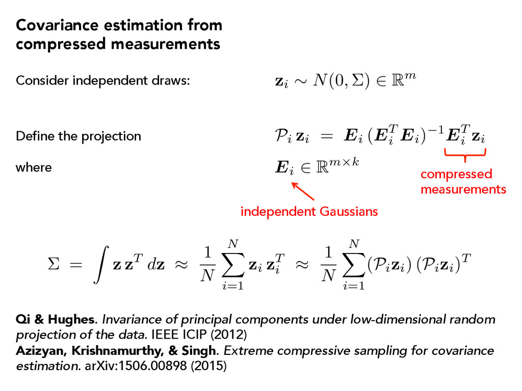
zT dz ⇡ 1 N N X i=1 zi zT i ⇡ 1 N N X i=1 (Pizi) (Pizi)T zi ⇠ N(0, ⌃) 2 Rm Pi zi = Ei (ET i Ei) 1ET i zi Consider independent draws: Define the projection Ei 2 Rm⇥k independent Gaussians Qi & Hughes. Invariance of principal components under low-dimensional random projection of the data. IEEE ICIP (2012) Azizyan, Krishnamurthy, & Singh. Extreme compressive sampling for covariance estimation. arXiv:1506.00898 (2015) compressed measurements
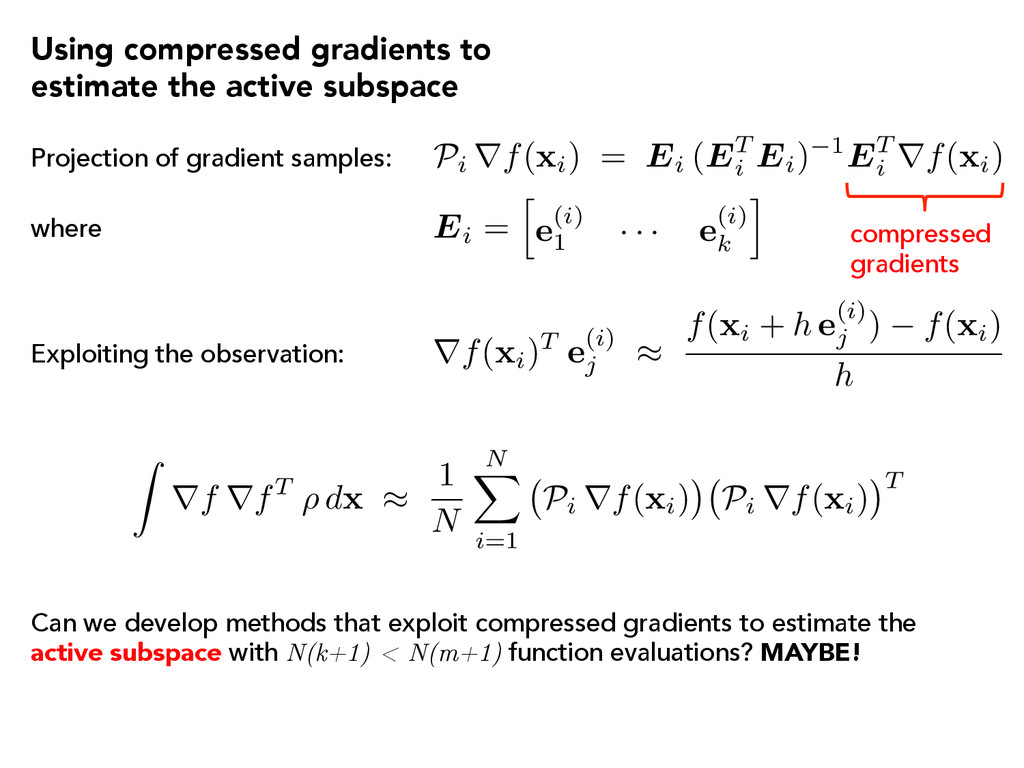
xi) = Ei (ET i Ei) 1ET i rf( xi) Ei = h e(i) 1 · · · e(i) k i rf( xi)T e (i) j ⇡ f( xi + h e (i) j ) f( xi) h Projection of gradient samples: where Exploiting the observation: Z rf rfT ⇢ d x ⇡ 1 N N X i=1 Pi rf( xi) Pi rf( xi) T Can we develop methods that exploit compressed gradients to estimate the active subspace with N(k+1) < N(m+1) function evaluations? MAYBE! compressed gradients
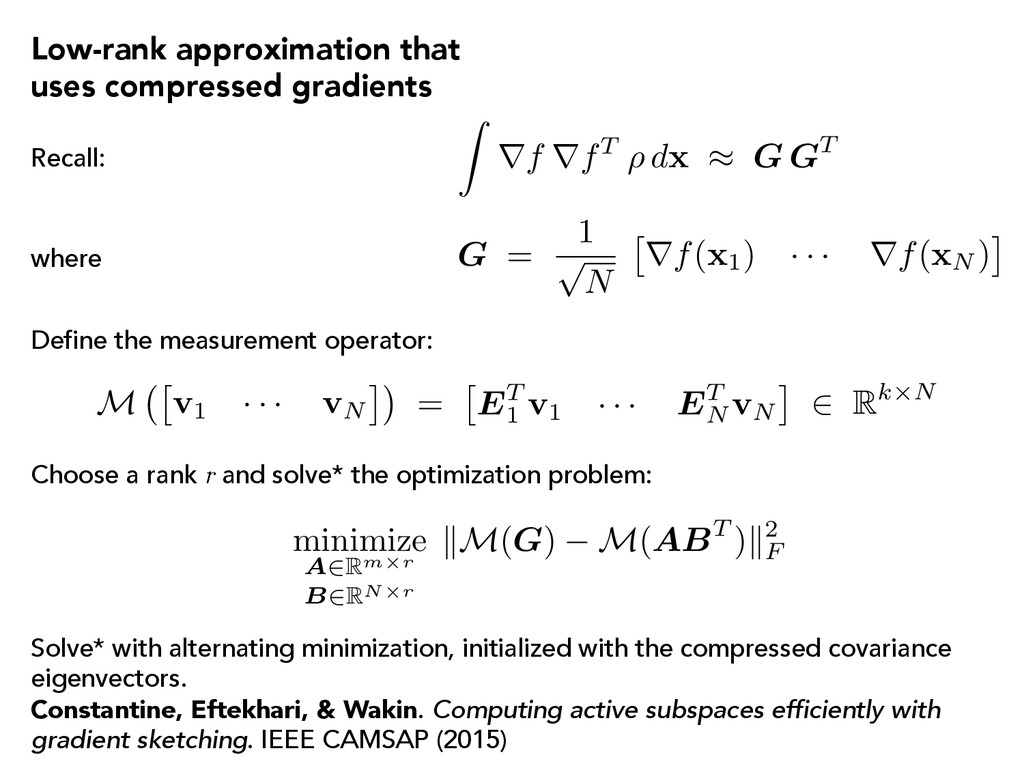
N ⇥ rf( x1) · · · rf( xN ) ⇤ M ⇥ v1 · · · vN ⇤ = ⇥ ET 1 v1 · · · ET N vN ⇤ 2 Rk⇥N Recall: Z rf rfT ⇢ d x ⇡ G GT where Define the measurement operator: minimize A2Rm⇥r B2RN⇥r kM(G) M(ABT )k2 F Choose a rank r and solve* the optimization problem: Solve* with alternating minimization, initialized with the compressed covariance eigenvectors. Constantine, Eftekhari, & Wakin. Computing active subspaces efficiently with gradient sketching. IEEE CAMSAP (2015)
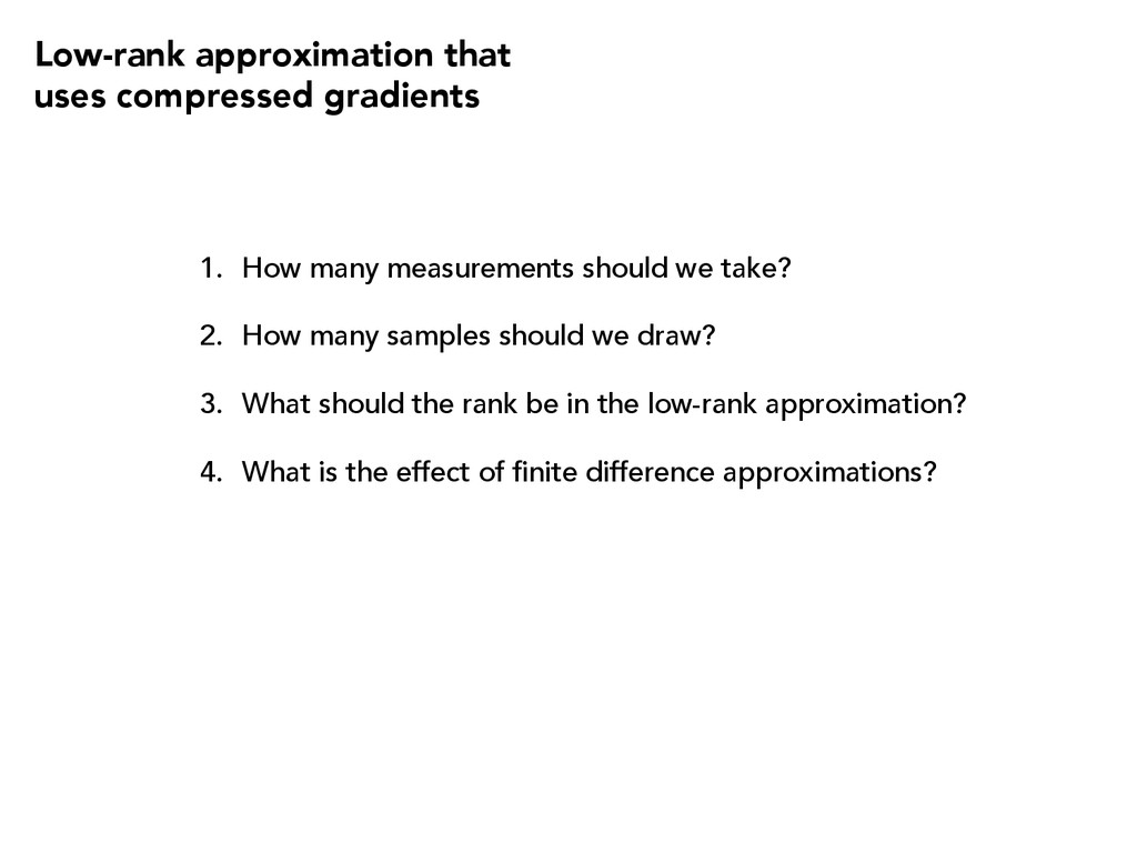
samples should we draw? 3. What should the rank be in the low-rank approximation? 4. What is the effect of finite difference approximations? Low-rank approximation that uses compressed gradients
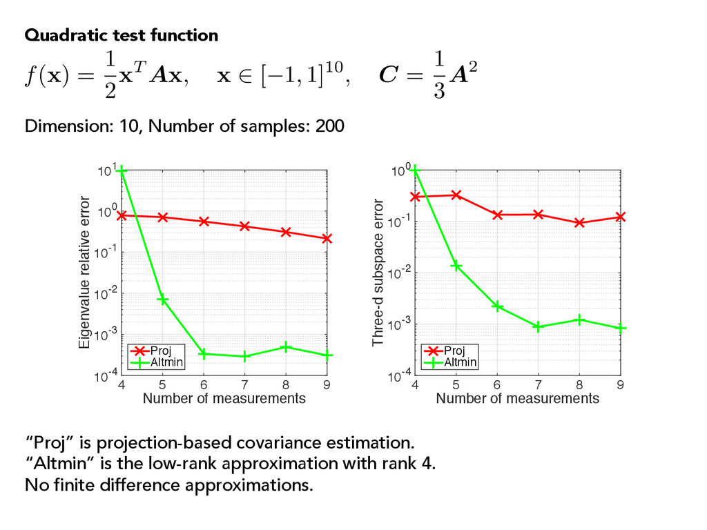
x 2 [ 1, 1]10, C = 1 3 A2 Number of measurements 4 5 6 7 8 9 Eigenvalue relative error 10-4 10-3 10-2 10-1 100 101 Proj Altmin Number of measurements 4 5 6 7 8 9 Three-d subspace error 10-4 10-3 10-2 10-1 100 Proj Altmin “Proj” is projection-based covariance estimation. “Altmin” is the low-rank approximation with rank 4. No finite difference approximations. Quadratic test function Dimension: 10, Number of samples: 200
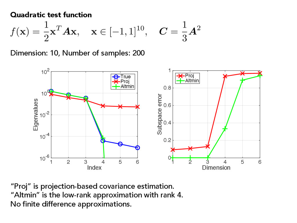
10-2 100 102 True Proj Altmin Dimension 1 2 3 4 5 6 Subspace error 0 0.2 0.4 0.6 0.8 1 Proj Altmin “Proj” is projection-based covariance estimation. “Altmin” is the low-rank approximation with rank 4. No finite difference approximations. f( x ) = 1 2x T A x , x 2 [ 1, 1]10, C = 1 3 A2 Quadratic test function Dimension: 10, Number of samples: 200
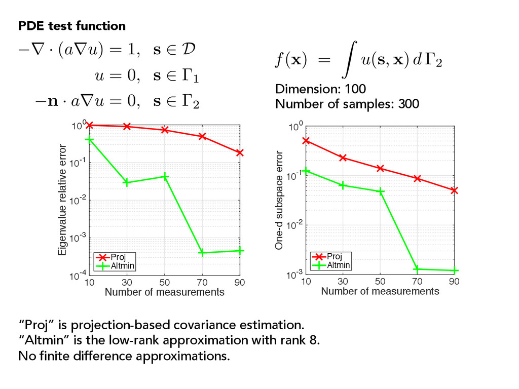
error 10-4 10-3 10-2 10-1 100 Proj Altmin Number of measurements 10 30 50 70 90 One-d subspace error 10-3 10-2 10-1 100 Proj Altmin “Proj” is projection-based covariance estimation. “Altmin” is the low-rank approximation with rank 8. No finite difference approximations. r · (aru) = 1, s 2 D u = 0, s 2 1 n · aru = 0, s 2 2 f( x ) = Z u( s , x ) d 2 PDE test function Dimension: 100 Number of samples: 300
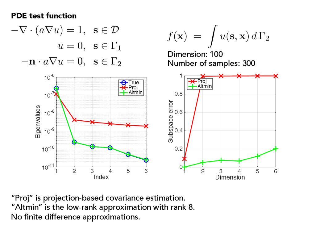
10-9 10-8 10-7 10-6 True Proj Altmin Dimension 1 2 3 4 5 6 Subspace error 0 0.2 0.4 0.6 0.8 1 Proj Altmin “Proj” is projection-based covariance estimation. “Altmin” is the low-rank approximation with rank 8. No finite difference approximations. r · (aru) = 1, s 2 D u = 0, s 2 1 n · aru = 0, s 2 2 f( x ) = Z u( s , x ) d 2 PDE test function Dimension: 100 Number of samples: 300
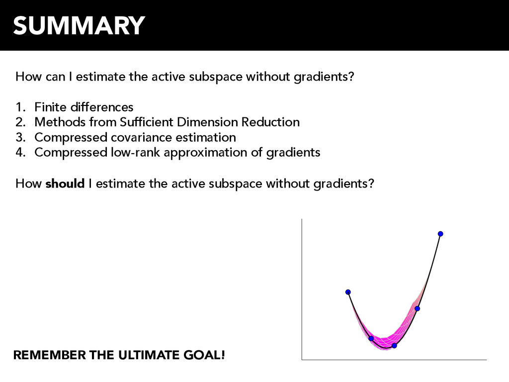
1. Finite differences 2. Methods from Sufficient Dimension Reduction 3. Compressed covariance estimation 4. Compressed low-rank approximation of gradients How should I estimate the active subspace without gradients? REMEMBER THE ULTIMATE GOAL!
• Is it really worth the effort to get the active subspace? PAUL CONSTANTINE Ben L. Fryrear Assistant Professor Colorado School of Mines activesubspaces.org! @DrPaulynomial! QUESTIONS?