Folding Unfolded - Polyglot - FP for Fun and Profit - Haskell and Scala - Part 2

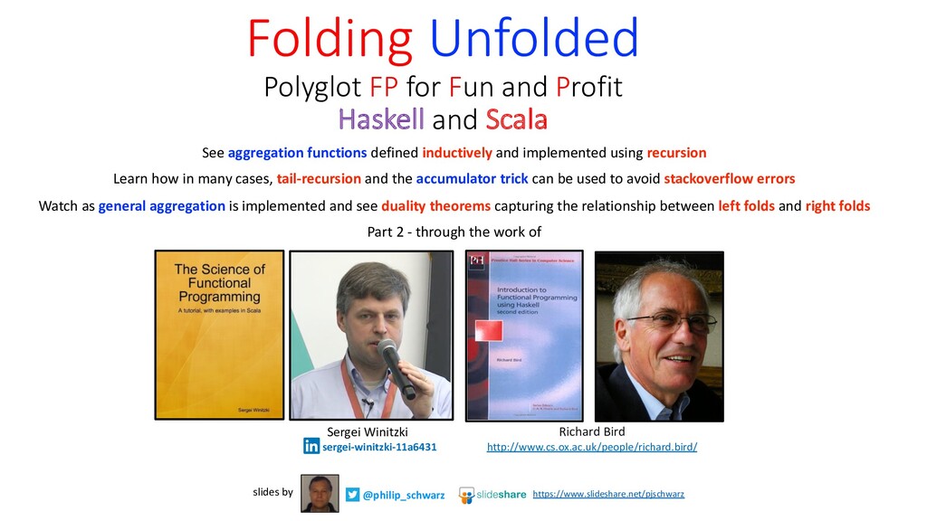
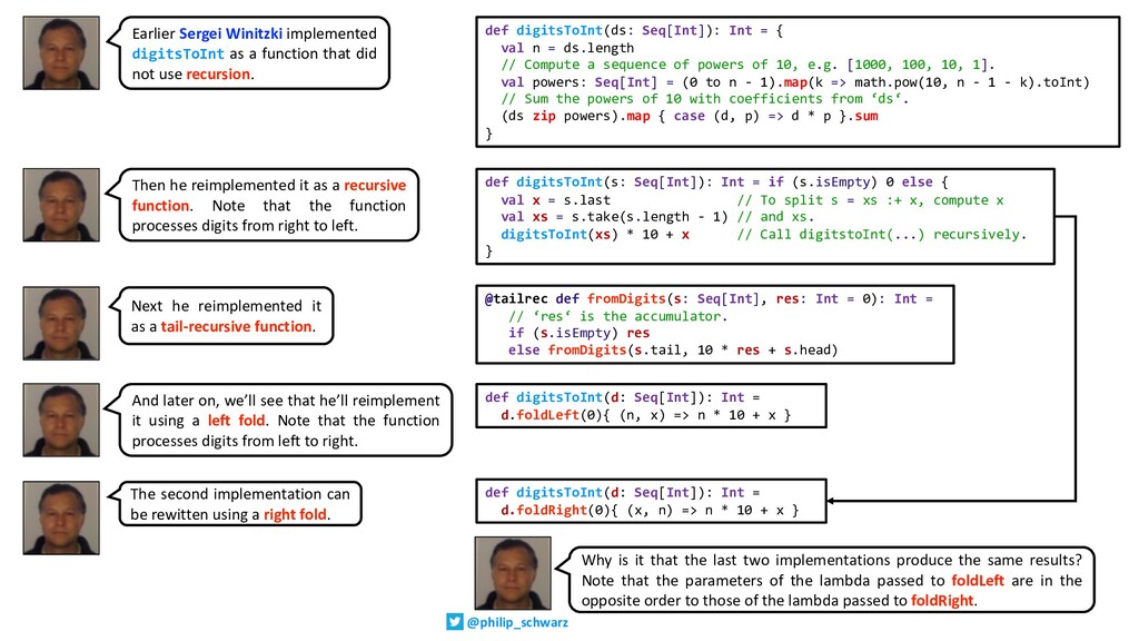
See aggregation functions defined inductively and implemented using recursion Learn
how in many cases, tail-recursion and the accumulator trick can be used to avoid stackoverflow errors Watch as general aggregation is implemented and see duality theorems capturing the relationship between left folds and right folds Part 2 - through the work of Folding Unfolded Polyglot FP for Fun and Profit Haskell and Scala @philip_schwarz slides by https://www.slideshare.net/pjschwarz Sergei Winitzki sergei-winitzki-11a6431 Richard Bird http://www.cs.ox.ac.uk/people/richard.bird/

While Part 1 was centred on Richard Bird’s Introduction to
Functional Programming using Haskell, Part 2 is centred on Sergei Winitzki’s The Science of Functional Programming. I hope Sergei will also forgive me for relying so heavily on his work, but I do not currently know of a better, a more comprehensive, or a more thorough introduction to folding. Sergei Winitzki sergei-winitzki-11a6431

Sergei Winitzki sergei-winitzki-11a6431 From the Preface: This book is at
once a reference text and a tutorial that teaches functional programmers how to reason mathematically about types and code, in a manner directly relevant to software practice. … The presentation is self-contained, defining and explaining all required ideas, notations, and Scala language features from scratch. The aim is to make all mathematical notions and derivations understandable. … The vision of this book is to explain the mathematical principles that guide the practice of functional programming — i.e. principles that help us write code. So, all mathematical developments in this book aremotivated and justified by practical programming issues and are accompanied by Scala code that illustrates their usage. … Each concept or technique is motivated and explained to make it as simple as possible (“but not simpler”) and also clarified via solved examples and exercises, which the readers will be able to solve after reading the chapter. … A software engineer needs to know only a few fragments of mathematical theory; namely, the fragments that answer questions arising in the practice of functional programming. So this book keeps theoretical material at the minimum; ars longa, vita brevis. … Mathematical generalizations are not pursued beyond proven practical relevance or immediate pedagogical usefulness. https://github.com/winitzki/sofp From the back cover: This book is a pedagogically developed series of in-depth tutorials on functional programming. The tutorials cover both the theory and the practice of functional programming, with the goal of building theoretical foundations that are valuable for practitioners. Long and difficult, yet boring explanations are given in excruciating detail. Solved examples and step-by-step derivations are followed by exercises for self-study.

Sergei Winitzki A software engineer needs to know only a
few fragments of mathematical theory; namely, the fragments that answer questions arising in the practice of functional programming. So this book keeps theoretical material at the minimum; ars longa, vita brevis.

2.2 Converting a sequence into a single value Until this
point, we have been working with sequences using methods such as .map and .zip. These techniques are powerful but still insufficient for solving certain problems. A simple computation that is impossible to do using .map is obtaining the sum of a sequence of numbers. The standard library method .sum already does this; but we cannot re-implement .sum ourselves by using .map, .zip, or .filter. These operations always compute new sequences, while we need to compute a single value (the sum of all elements) from a sequence. We have seen a few library methods such as .count, .length, and .max that compute a single value from a sequence; but we still cannot implement .sum using these methods. What we need is a more general way of converting a sequence to a single value, such that we could ourselves implement .sum, .count, .max, and other similar computations. Another task not solvable with .map, .sum, etc., is to compute a floating-point number from a given sequence of decimal digits (including a “dot” character): def digitsToDouble(ds: Seq[Char]): Double = ??? scala> digitsToDouble(Seq(’2’, ’0’, ’4’, ’.’, ’5’)) res0: Double = 204.5 Why is it impossible to implement this function using .map, .sum, and other methods we have seen so far? In fact, the same task for integer numbers (instead of floating-point numbers) can be implemented via .length, .map, .sum, and .zip: def digitsToInt(ds: Seq[Int]): Int = { val n = ds.length // Compute a sequence of powers of 10, e.g. [1000, 100, 10, 1]. val powers: Seq[Int] = (0 to n - 1).map(k => math.pow(10, n - 1 - k).toInt) // Sum the powers of 10 with coefficients from ‘ds‘. (ds zip powers).map { case (d, p) => d * p }.sum } scala> digitsToInt(Seq(2,4,0,5)) res0: Int = 2405 Sergei Winitzki sergei-winitzki-11a6431

Yes, well spotted: we have already seen the problem that
is solved by digitsToInt in Part 1. suppose we want a function that takes a list of digits and returns the corresponding decimal number; thus [0 , 1 , … , n ] = ∑!"# $ 10($&!) It is assumed that the most significant digit comes first in the list.

This task is doable because the required computation can be
written as the formula = 2 !"# $&( ∗ 10$&(&!. The sequence of powers of 10 can be computed separately and “zipped” with the sequence of digits . However, for floating- point numbers, the sequence of powers of 10 depends on the position of the “dot” character. Methods such as .map or .zip cannot compute a sequence whose next elements depend on previous elements, and the dependence is described by some custom function. 2.2.1 Inductive definitions of aggregation functions Mathematical induction is a general way of expressing the dependence of next values on previously computed values. To define a function from a sequence to a single value (e.g. an aggregation function f:Seq[Int] => Int) via mathematical induction, we need to specify two computations: • (The base case of the induction.) We need to specify what value the function f returns for an empty sequence, Seq(). The standard method isEmpty can be used to detect empty sequences. In case the function f is only defined for non-empty sequences, we need to specify what the function f returns for a one-element sequence such as Seq(x), with any x. • (The inductive step.) Assuming that the function f is already computed for some sequence xs (the inductive assumption), how to compute the function f for a sequence with one more element x? The sequence with one more element is written as xs :+ x. So, we need to specify how to compute f(xs :+ x) assuming that f(xs) is already known. Once these two computations are specified, the function f is defined (and can in principle be computed) for an arbitrary input sequence. This is how induction works in mathematics, and it works in the same way in functional programming. With this approach, the inductive definition of the method .sum looks like this: • The sum of an empty sequence is 0. That is, Seq().sum == 0. • If the result is already known for a sequence xs, and we have a sequence that has one more element x, the new result is equal to xs.sum + x. In code, this is (xs :+ x).sum == xs.sum + x. Sergei Winitzki sergei-winitzki-11a6431

The inductive definition of the function digitsToInt is: • For
an empty sequence of digits, Seq(), the result is 0. This is a convenient base case, even if we never call digitsToInt on an empty sequence. • If digitsToInt(xs) is already known for a sequence xs of digits, and we have a sequence xs :+ x with one more digit x, then digitsToInt(xs :+ x) = digitsToInt(xs) * 10 + x Let us write inductive definitions for methods such as .length, .max, and .count: • The length of a sequence: – for an empty sequence, Seq().length == 0 – if xs.length is known then (xs :+ x).length == xs.length + 1 • Maximum element of a sequence (undefined for empty sequences): – for a one-element sequence, Seq(x).max == x – if xs.max is known then (xs :+ x).max == math.max(xs.max, x) • Count the sequence elements satisfying a predicate p: – for an empty sequence, Seq().count(p) == 0 – if xs.count(p) is known then (xs :+ x).count(p) == xs.count(p) + c, where we set c = 1 when p(x) == true and c = 0 otherwise There are two main ways of translating mathematical induction into code. The first way is to write a recursive function. The second way is to use a standard library function, such as foldLeft or reduce. Most often it is better to use the standard library functions, but sometimes the code is more transparent when using explicit recursion. So let us consider each of these ways in turn. Sergei Winitzki sergei-winitzki-11a6431

2.2.2 Implementing functions by recursion A recursive function is any
function that calls itself somewhere within its own body. The call to itself is the recursive call. When the body of a recursive function is evaluated, it may repeatedly call itself with different arguments until the result value can be computed without any recursive calls. The last recursive call corresponds to the base case of the induction. It is an error if the base case is never reached, as in this example: scala> def infiniteLoop(x: Int): Int = infiniteLoop(x+1) infiniteLoop : (x: Int)Int scala> infiniteLoop(2) // You will need to press Ctrl-C to stop this. We translate mathematical induction into code by first writing a condition to decide whether we have the base case or the inductive step. As an example, let us define .sum by recursion. The base case returns 0, and the inductive step returns a value computed from the recursive call: def sum(s: Seq[Int]): Int = if (s.isEmpty) 0 else { val x = s.head // To split s = x +: xs, compute x val xs = s.tail // and xs. sum(xs) + x // Call sum(...) recursively. } In this example, the if/else expression will separate the base case from the inductive step. In the inductive step, it is convenient to split the given sequence s into its first element x, or the head of s, and the remainder tail sequence xs. So, we split s as s = x +: xs rather than as s = xs :+ x (footnote: It is easier to remember the meaning of x +: xs and xs :+ x if we note that the colon always points to the collection). For computing the sum of a numerical sequence, the order of summation does not matter. However, the order of operations will matter for many other computational tasks. We need to choose whether the inductive step should split the sequence as s = x +: xs or as s = xs :+ x, according to the task at hand. Sergei Winitzki sergei-winitzki-11a6431

Consider the implementation of digitsToInt according to the inductive definition
shown in the previous subsection: def digitsToInt(s: Seq[Int]): Int = if (s.isEmpty) 0 else { val x = s.last // To split s = xs :+ x, compute x val xs = s.take(s.length - 1) // and xs. digitsToInt(xs) * 10 + x // Call digitstoInt(...) recursively. } In this example, it is important to split the sequence into s = xs :+ x in this order, and not in the order x +: xs. The reason is that digits increase their numerical value from right to left, so we need to multiply the value of the left subsequence, digitsToInt(xs), by 10, in order to compute the correct result. These examples show how mathematical induction is converted into recursive code. This approach often works but has two technical problems. The first problem is that the code will fail due to a “stack overflow” when the input sequence s is long enough. In the next subsection, we will see how this problem is solved (at least in some cases) using “tail recursion”. The second problem is that each inductively defined function repeats the code for checking the base case and the code for splitting the sequence s into the subsequence xs and the extra element x. This repeated common code can be put into a library function, and the Scala library provides such functions. We will look at using them in Section 2.2.4. The inductive definition of the function digitsToInt is: • For an empty sequence of digits, Seq(), the result is 0. This is a convenient base case, even if we never call digitsToInt on an empty sequence. • If digitsToInt(xs) is already known for a sequence xs of digits, and we have a sequence xs :+ x with one more digit x, then digitsToInt(xs :+ x) = digitsToInt(xs) * 10 + x Sergei Winitzki sergei-winitzki-11a6431

def digitsToInt(s: Seq[Int]): Int = if (s.isEmpty) 0 else {
val x = s.last // To split s = xs :+ x, compute x val xs = s.take(s.length - 1) // and xs. digitsToInt(xs) * 10 + x // Call digitstoInt(...) recursively. } def sum(s: Seq[Int]): Int = if (s.isEmpty) 0 else { val x = s.head // To split s = x +: xs, compute x val xs = s.tail // and xs. sum(xs) + x // Call sum(...) recursively. } For computing the sum of a numerical sequence, the order of summation does not matter. However, the order of operations will matter for many other computational tasks. We need to choose whether the inductive step should split the sequence as s = x +: xs or as s = xs :+ x, according to the task at hand. This slide, which repeats the definitions of sum and digitsToInt, is just here to reinforce the idea that in many tasks, the order of operations matters. Sergei Winitzki

val x = s.last // To split s = xs :+ x, compute x val xs = s.take(s.length - 1) // and xs. digitsToInt(xs) * 10 + x // Call digitstoInt(...) recursively. } To illustrate, suppose we want a function decimal that takes a list of digits and returns the corresponding decimal number; thus [0 , 1 , … , n ] = ∑!"# $ 10($&!) It is assumed that the most significant digit comes first in the list. One way to compute decimal efficiently is by a process of multiplying each digit by ten and adding in the following digit. For example 0 , 1 , 2 = 10 × 10 × 10 × 0 + 0 + 1 + 2 This decomposition of a sum of powers is known as Horner’s rule. Yes, this solution is an implementation of the rule we saw in Part 1

2.2.3 Tail recursion The code of lengthS will fail for
large enough sequences. To see why, consider an inductive definition of the .length method as a function lengthS: def lengthS(s: Seq[Int]): Int = if (s.isEmpty) 0 else 1 + lengthS(s.tail) scala> lengthS((1 to 1000).toList) res0: Int = 1000 scala> val s = (1 to 100_000).toList s : List[Int] = List(1, 2, 3, 4, 5, 6, 7, 8, 9, 10, 11, 12, 13, 14, 15, 16, 17, 18, 19, 20, 21, 22, 23, 24, 25, 26, 27, 28, 29, 30, 31, 32, ... scala> lengthS(s) java.lang.StackOverflowError at .lengthS(<console>:12) at .lengthS(<console>:12) at .lengthS(<console>:12) at .lengthS(<console>:12) ... The problem is not due to insufficient main memory: we are able to compute and hold in memory the entire sequence s. The problem is with the code of the function lengthS. This function calls itself inside the expression 1 + lengthS(...). So we can visualize how the computer evaluates this code: lengthS(Seq(1, 2, ..., 100000)) = 1 + lengthS(Seq(2, ..., 100000)) = 1 + (1 + lengthS(Seq(3, ..., 100000))) = ... Sergei Winitzki sergei-winitzki-11a6431

The function body of lengthS will evaluate the inductive step,
that is, the “else” part of the “if/else”, about 100_000 times. Each time, the sub-expression with nested computations 1+(1+(...)) will get larger. This intermediate sub-expression needs to be held somewhere in memory, until at some point the function body goes into the base case and returns a value. When that happens, the entire intermediate sub-expression will contain about 100_000_nested function calls still waiting to be evaluated. This sub-expression is held in a special area of memory called stack memory, where the not-yet-evaluated nested function calls are held in the order of their calls, as if on a “stack”. Due to the way computer memory is managed, the stack memory has a fixed size and cannot grow automatically. So, when the intermediate expression becomes large enough, it causes an overflow of the stack memory and crashes the program. A way to avoid stack overflows is to use a trick called tail recursion. Using tail recursion means rewriting the code so that all recursive calls occur at the end positions (at the “tails”) of the function body. In other words, each recursive call must be itself the last computation in the function body, rather than placed inside other computations. Here is an example of tail-recursive code: def lengthT(s: Seq[Int], res: Int): Int = if (s.isEmpty) res else lengthT(s.tail, 1 + res) In this code, one of the branches of the if/else returns a fixed value without doing any recursive calls, while the other branch returns the result of a recursive call to lengthT(...). In the code of lengthT, recursive calls never occur within any sub- expressions. def lengthS(s: Seq[Int]): Int = if (s.isEmpty) 0 else 1 + lengthS(s.tail) lengthS(Seq(1, 2, ..., 100000)) = 1 + lengthS(Seq(2, ..., 100000)) = 1 + (1 + lengthS(Seq(3, ..., 100000))) = ... Sergei Winitzki sergei-winitzki-11a6431

It is not a problem that the recursive call to
lengthT has some sub-expressions such as 1 + res as its arguments, because all these sub-expressions will be computed before lengthT is recursively called. The recursive call to lengthT is the last computation performed by this branch of the if/else. A tail-recursive function can have many if/else or match/case branches, with or without recursive calls; but all recursive calls must be always the last expressions returned. The Scala compiler has a feature for checking automatically that a function’s code is tail-recursive : the @tailrec annotation. If a function with a @tailrec annotation is not tail-recursive, or is not recursive at all, the program will not compile. @tailrec def lengthT(s: Seq[Int], res: Int): Int = if (s.isEmpty) res else lengthT(s.tail, 1 + res) Let us trace the evaluation of this function on an example: lengthT(Seq(1,2,3), 0) = lengthT(Seq(2,3), 1 + 0) // = lengthT(Seq(2,3), 1) = lengthT(Seq(3), 1 + 1) // = lengthT(Seq(3), 2) = lengthT(Seq(), 1 + 2) // = lengthT(Seq(), 3) = 3 All sub-expressions such as 1 + 1 and 1 + 2 are computed before recursive calls to lengthT. Because of that, sub-expressions do not grow within the stack memory. This is the main benefit of tail recursion. How did we rewrite the code of lengthS to obtain the tail-recursive code of lengthT? An important difference between lengthS and lengthT is the additional argument, res, called the accumulator argument. This argument is equal to an intermediate result of the computation. The next intermediate result (1 + res) is computed and passed on to the next recursive call via the accumulator argument. In the base case of the recursion, the function now returns the accumulated result, res, rather than 0, because at that time the computation is finished. Rewriting code by adding an accumulator argument to achieve tail recursion is called the accumulator technique or the “accumulator trick”. def lengthS(s: Seq[Int]): Int = if (s.isEmpty) 0 else 1 + lengthS(s.tail) Sergei Winitzki sergei-winitzki-11a6431

One consequence of using the accumulator trick is that the
function lengthT now always needs a value for the accumulator argument. However, our goal is to implement a function such as length(s) with just one argument, s:Seq[Int]. We can define length(s) = lengthT(s, ???) if we supply an initial accumulator value. The correct initial value for the accumulator is 0, since in the base case (an empty sequence s) we need to return 0. So, a tail-recursive implementation of lengthT requires us to define two functions: the tail-recursive lengthT and an “adapter” function that will set the initial value of the accumulator argument. To emphasize that lengthT is a helper function, one could define it inside the adapter function: def length[A](s: Seq[A]): Int = { @tailrec def lengthT(s: Seq[A], res: Int): Int = { if (s.isEmpty) res else lengthT(s.tail, 1 + res) } lengthT(s, 0) } When length is implemented like that, users will not be able to call lengthT directly, because it is only visible within the body of the length function. Another possibility in Scala is to use a default value for the res argument: @tailrec def length(s: Seq[A], res: Int = 0): Int = if (s.isEmpty) res else length(s.tail, 1 + res) Giving a default value for a function argument is the same as defining two functions: one with that argument and one without. For example, the syntax def f(x: Int, y: Boolean = false): Int = ... // Function body. Sergei Winitzki sergei-winitzki-11a6431

is equivalent to defining two functions (with the same name),
def f(x: Int, y: Boolean) = ... // Function body. def f(x: Int): Int = f(Int, false) Using a default argument value, we can define the tail-recursive helper function and the adapter function at once, making the code shorter. The accumulator trick works in a large number of cases, but it may be far from obvious how to introduce the accumulator argument, what its initial value must be, and how to define the inductive step for the accumulator. In the example with the lengthT function, the accumulator trick works because of the following mathematical property of the expression being computed: 1 + (1 + (1 + (... + 1))) = (((1 + 1) + 1) + ...) + 1 . This is the associativity law of addition. Due to that law, the computation can be rearranged so that additions associate to the left. In code, it means that intermediate expressions are computed immediately before making recursive calls; this avoids the growth of the intermediate expressions. Usually, the accumulator trick works because some associativity law is present. In that case, we are able to rearrange the order of recursive calls so that these calls always occur outside all other subexpressions, — that is, in tail positions. However, not all computations obey a suitable associativity law. Even if a code rearrangement exists, it may not be immediately obvious how to find it. Sergei Winitzki sergei-winitzki-11a6431

val x = s.last // To split s = xs :+ x, compute x val xs = s.take(s.length - 1) // and xs. digitsToInt(xs) * 10 + x // Call digitstoInt(...) recursively. } As an example, consider a tail-recursive re-implementation of the function digitsToInt from the previous subsection where the recursive call is within a sub-expression digitsToInt(xs) * 10 + x. To transform the code into a tail-recursive form, we need to rearrange the main computation, r = dn−1 + 10 ∗ (dn−2 +10 ∗ (dn−3 + 10 ∗ (...d0 ))) so that the operations group to the left. We can do this by rewriting r as r = ((d0 ∗ 10 + d1 ) ∗ 10 + ...) ∗ 10 + dn−1 It follows that the digit sequence s must be split into the leftmost digit and the rest, s = s.head +: s.tail. So, a tail-recursive implementation of the above formula is @tailrec def fromDigits(s: Seq[Int], res: Int = 0): Int = // ‘res‘ is the accumulator. if (s.isEmtpy) res else fromDigits(s.tail, 10 * res + s.head) Despite a certain similarity between this code and the code of digitsToInt from the previous subsection, the implementation fromDigits cannot be directly derived from the inductive definition of digitsToInt. One needs a separate proof that fromDigits(s, 0) computes the same result as digitsToInt(s). The proof follows from the following property. Statement 2.2.3.1 For any xs: Seq[Int] and r: Int, we have fromDigits(xs, r) = digitsToInt(xs) + r * math.pow(10, s.length) Proof We prove this by induction. <…proof omitted…> Sergei Winitzki sergei-winitzki-11a6431 not tail-recursive

To illustrate, suppose we want a function decimal that takes
a list of digits and returns the corresponding decimal number; thus [0 , 1 , … , n ] = ∑!"# $ 10($&!) It is assumed that the most significant digit comes first in the list. One way to compute decimal efficiently is by a process of multiplying each digit by ten and adding in the following digit. For example 0 , 1 , 2 = 10 × 10 × 10 × 0 + 0 + 1 + 2 This decomposition of a sum of powers is known as Horner’s rule. Suppose we define ⊕ by ⊕ = 10 × + . Then we can rephrase the above equation as 0 , 1 , 2 = (0 ⊕ 0 ) ⊕ 1 ⊕ 2 @tailrec def fromDigits(s: Seq[Int], res: Int = 0): Int = // ‘res‘ is the accumulator. if (s.isEmpty) res else fromDigits(s.tail, 10 * res + s.head) Yes, this solution uses the ⊕ function and the ‘rephrased’ equation we saw in Part 1

2.2.4 Implementing general aggregation (foldLeft) An aggregation converts a sequence
of values into a single value. In general, the type of the result may be different from the type of sequence elements. To describe that general situation, we introduce type parameters, A and B, so that the input sequence is of type Seq[A] and the aggregated value is of type B. Then an inductive definition of any aggregation function f: Seq[A] => B looks like this: • (Base case.) For an empty sequence, f(Seq()) = b0 where b0:B is a given value. • (Inductive step.) Assuming that f(xs) = b is already computed, we define f(xs :+ x) = g(x, b) where g is a given function with type signature g:(A, B) => B. The code implementing f is written using recursion: def f[A, B](s: Seq[A]): B = if (s.isEmpty) b0 else g(s.last, f(s.take(s.length - 1))) We can now refactor this code into a generic utility function, by making b0 and g into parameters. A possible implementation is def f[A, B](s: Seq[A], b: B, g: (A, B) => B): B = if (s.isEmpty) b else g(s.last, f(s.take(s.length - 1), b, g) However, this implementation is not tail-recursive. Sergei Winitzki sergei-winitzki-11a6431

Applying f to a sequence of, say, three elements, Seq(x,
y, z), will create an intermediate expression g(z, g(y, g(x, b))). This expression will grow with the length of s, which is not acceptable. To rearrange the computation into a tail-recursive form, we need to start the base case at the innermost call g(x, b), then compute g(y, g(x, b)) and continue. In other words, we need to traverse the sequence starting from its leftmost element x, rather than starting from the right. So, instead of splitting the sequence s into s.take(s.length - 1) :+ s.last as we did in the code of f, we need to split s into s.head :+ s.tail. Let us also exchange the order of the arguments of g, in order to be more consistent with the way this code is implemented in the Scala library. The resulting code is tail-recursive: @tailrec def leftFold[A, B](s: Seq[A], b: B, g: (B, A) => B): B = if (s.isEmpty) b else leftFold(s.tail, g(b, s.head), g) We call this function a “left fold” because it aggregates (or “folds”) the sequence starting from the leftmost element. In this way, we have defined a general method of computing any inductively defined aggregation function on a sequence. The function leftFold implements the logic of aggregation defined via mathematical induction. Using leftFold, we can write concise implementations of methods such as .sum, .max, and many other aggregation functions. The method leftFold already contains all the code necessary to set up the base case and the inductive step. The programmer just needs to specify the expressions for the initial value b and for the updater function g. def f[A, B](s: Seq[A], b: B, g: (A, B) => B): B = if (s.isEmpty) b else g(s.last, f(s.take(s.length - 1), b, g) Sergei Winitzki sergei-winitzki-11a6431

I think it is worth repeating some of what we
just saw on the previous slide, so it sinks in better Sergei Winitzki @tailrec def leftFold[A, B](s: Seq[A], b: B, g: (B, A) => B): B = if (s.isEmpty) b else leftFold(s.tail, g(b, s.head), g) We call this function a “left fold” because it aggregates (or “folds”) the sequence starting from the leftmost element. In this way, we have defined a general method of computing any inductively defined aggregation function on a sequence. The function leftFold implements the logic of aggregation defined via mathematical induction. Using leftFold, we can write concise implementations of methods such as .sum, .max, and many other aggregation functions. The method leftFold already contains all the code necessary to set up the base case and the inductive step. The programmer just needs to specify the expressions for the initial value b and for the updater function g.

As a first example, let us use leftFold for implementing
the .sum method: def sum(s: Seq[Int]): Int = leftFold(s, 0, { (x, y) => x + y }) To understand in detail how leftFold works, let us trace the evaluation of this function when applied to Seq(1, 2, 3): // Here, g = { (x, y) => x + y }, so g(x, y) = x + y. == leftFold(Seq(2, 3), g(0, 1), g) // g (0, 1) = 1. == leftFold(Seq(2, 3), 1, g) // Now expand the code of ‘leftFold‘. == leftFold(Seq(3), g(1, 2), g) // g(1, 2) = 3; expand the code. == leftFold(Seq(), g(3, 3), g) // g(3, 3) = 6; expand the code. == 6 The second argument of leftFold is the accumulator argument. The initial value of the accumulator is specified when first calling leftFold. At each iteration, the new accumulator value is computed by calling the updater function g, which uses the previous accumulator value and the value of the next sequence element. To visualize the process of recursive evaluation, it is convenient to write a table showing the sequence elements and the accumulator values as they are updated: We implemented leftFold only as an illustration. Scala’s library has a method called .foldLeft implementing the same logic using a slightly different type signature. To see this difference, compare the implementation of sum using our leftFold function and using the standard .foldLeft method: def sum(s: Seq[Int]): Int = leftFold(s, 0, { (x, y) => x + y }) def sum(s: Seq[Int]): Int = s.foldLeft(0) { (x, y) => x + y } Current element x Old accumulator value New accumulator value 1 0 1 2 1 3 3 3 6 Sergei Winitzki sergei-winitzki-11a6431

The syntax of .foldLeft makes it more convenient to use
a nameless function as the updater argument of .foldLeft, since curly braces separate that argument from others. We will use the standard .foldLeft method from now on. In general, the type of the accumulator value can be different from the type of the sequence elements. An example is an implementation of count: def count[A](s: Seq[A], p: A => Boolean): Int = s.foldLeft(0) { (x, y) => x + (if (p(y)) 1 else 0) } The accumulator is of type Int, while the sequence elements can have an arbitrary type, parameterized by A. The .foldLeft method works in the same way for all types of accumulators and all types of sequence elements. The method .foldLeft is available in the Scala library for all collections, including dictionaries and sets. Since .foldLeft is tail- recursive, no stack overflows will occur even for very large sequences. The Scala library contains several other methods similar to .foldLeft, such as .foldRight and .reduce. (However, .foldRight is not tail-recursive!) def sum(s: Seq[Int]): Int = leftFold(s, 0, { (x, y) => x + y }) def sum(s: Seq[Int]): Int = s.foldLeft(0) { (x, y) => x + y } Sergei Winitzki sergei-winitzki-11a6431

In Introduction to Functional Programming using Haskell, there is a
section covering the laws of fold, which include three duality theorems. 4.6 Laws of fold There are a number of important laws concerning and its relationship with . As we saw in section 3.3, instead of having to prove a property of a recursive function over a recursive datatype by writing down an explicit induction proof, one can often phrase the property as an instance of one of the laws of the operator for the datatype. 4.6.1 Duality theorems The first three laws are called duality theorems and concern the relationship between and . What we are going to do in the next seven slides is look back at three of the functions that Sergei Winitzki discussed in his book, and relate them to the three duality theorems. @philip_schwarz

We translate mathematical induction into code by first writing a
condition to decide whether we have the base case or the inductive step. As an example, let us define .sum by recursion. The base case returns 0, and the inductive step returns a value computed from the recursive call: def sum(s: Seq[Int]): Int = if (s.isEmpty) 0 else { val x = s.head // To split s = x +: xs, compute x val xs = s.tail // and xs. sum(xs) + x // Call sum(...) recursively. } In this example, the if/else expression will separate the base case from the inductive step. In the inductive step, it is convenient to split the given sequence s into its first element x, or the head of s, and the remainder tail sequence xs. So, we split s as s = x +: xs rather than as s = xs :+ x For computing the sum of a numerical sequence, the order of summation does not matter. Remember earlier when Sergei Winitzki explained that for computing the sum of a numerical sequence, the order of summation does not matter? If the order of summation doesn’t matter, does that mean that it is possible to implement the sum function both using a right fold and using a left fold? The answer is yes, but with the qualification mentioned on the nexts slide. Sergei Winitzki

def foldr[A,B](f: (A,B) => B)(e: B)(s: List[A]): B = s
match { case Nil => e case x::xs => f(x,foldr(f)(e)(xs)) } def foldl[A,B](f: (B,A) => B)(e: B) (s: List[A]): B = s match { case Nil => e case x::xs => foldl(f)(f(e,x))(xs) } def add(x: Int, y: Int): Int = x + y def sumr(s: List[Int]): Int = foldr(add)(0)(s) def suml(s: List[Int]): Int = foldl(add)(0)(s) assert( sumr(List(1,2,3,4,5)) == 15) assert( suml(List(1,2,3,4,5)) == 15) That works: we get the same result. But if we pass foldr a sufficiently large sequence, it encounters a stack overflow error, since foldr is not tail-recursive. val oneTo40K = List.range(1,40_000) assert( suml(oneTo40K) == 799_980_000) assert( try { sumr(oneTo40K) false } catch { case _:StackOverflowError => true } ) First, let’s define foldr and foldl. Yes we are using List[A] rather than Seq[A], simply to be consistent with the foldr and foldl definitions seen in in Part 1 (we’ll be doing so throughout the slides on the duality theorems). Next, let’s define sumr using foldr and suml using foldl. @philip_schwarz We had already seen the Scala version of foldr in Part1, but not of foldl.

First duality theorem. Suppose ⊕ is associative with unit .
Then ⊕ = ⊕ For all finite lists . For example, we could have defined = + 0 and = (⋀) concat = (⧺) [ ] However, as we will elaborate in chapter 7, it is sometimes more efficient to implement a function using , and sometimes more efficient to use . The reason why foldr(add)(0)(s) produces the same result as foldl(add)(0)(s) (except when foldr overflows the stack, of course), is that addition, 0 and s satisfy the constraints of the first duality theorem, in that addition is an associative operation, 0 is the unit of addition, and s is a finite sequence. e.g. see the slide after next for how the efficiency of is affected by whether it is implemented using or . ∷ → → → → → = ∶ = ∷ → → → → → = ∶ = def foldr[A,B](f: (A,B) => B)(e: B)(s: List[A]): B = s match { case Nil => e case x::xs => f(x,foldr(f)(e)(xs)) } def foldl[A,B](f: (B,A) => B)(e: B) (s: List[A]): B = s match { case Nil => e case x::xs => foldl(f)(f(e,x))(xs) }

def lengthS(s: Seq[Int]): Int = if (s.isEmpty) 0 else 1
+ lengthS(s.tail) @tailrec def length(s: Seq[A], res: Int = 0): Int = if (s.isEmpty) res else length(s.tail, 1 + res) Remember earlier when Sergei Winitzki first implemented a lengthS function that was not tail-recursive and then implemented a length function that was tail recursive? Let’s implement the first function using foldr and the second function using foldl. def lengthr[A](s: List[A]): Int = { def onePlus(a: A, n: Int): Int = 1 + n foldr(onePlus)(0)(s) } def lengthl[A](s: List[A]): Int = { def plusOne(n: Int, a: A): Int = 1 + n foldl(plusOne)(0)(s) } That works: we get the same result. assert( lengthr(List(1,2,3,4,5)) == 5) assert( lengthl(List(1,2,3,4,5)) == 5)

The reason why foldr(onePlus)(0)(s) produces the same result as foldl(plusOne)(0)(s)
(except when foldr overflows the stack, of course), is that onePlus, plusOne, 0, and s satisfy the constraints of the second duality theorem. Second duality theorem. This is a generalization of the first. Suppose ⊕, ⊗, and are such that for all , , and we have ⊕ ⊗ = ⊕ ⊗ ⊕ = ⊗ In other words, ⊕ and ⊗ associate with each other, and on the right of ⊕ is equivalent to on the left of ⊗. Then ⊕ = ⊗ For all finite lists . … The second duality theorem has the first duality theorem as a special case, namely when ⊕ = ⊗ To illustrate the second duality theorem, consider the following definitions ℎ ∷ [α] → ℎ = 0, = 1 + ℎ = 0, = + 1 reverse ∷ α → [α] reverse = , = ⧺ [] reverse = , = : The functions , , and 0 meet the conditions of the second duality theorem, as do , , and . We leave the verification as an exercise. Hence the two definitions of ℎ and reverse are equivalent on all finite lists. It is not obvious whether there is any practical difference between the two definitions of ℎ, but the second program for reverse is the more efficient of the two.

Earlier Sergei Winitzki implemented digitsToInt as a function that did
not use recursion. def digitsToInt(ds: Seq[Int]): Int = { val n = ds.length // Compute a sequence of powers of 10, e.g. [1000, 100, 10, 1]. val powers: Seq[Int] = (0 to n - 1).map(k => math.pow(10, n - 1 - k).toInt) // Sum the powers of 10 with coefficients from ‘ds‘. (ds zip powers).map { case (d, p) => d * p }.sum } def digitsToInt(s: Seq[Int]): Int = if (s.isEmpty) 0 else { val x = s.last // To split s = xs :+ x, compute x val xs = s.take(s.length - 1) // and xs. digitsToInt(xs) * 10 + x // Call digitstoInt(...) recursively. } @tailrec def fromDigits(s: Seq[Int], res: Int = 0): Int = // ‘res‘ is the accumulator. if (s.isEmpty) res else fromDigits(s.tail, 10 * res + s.head) Then he reimplemented it as a recursive function. Note that the function processes digits from right to left. Next he reimplemented it as a tail-recursive function. And later on, we’ll see that he’ll reimplement it using a left fold. Note that the function processes digits from left to right. def digitsToInt(d: Seq[Int]): Int = d.foldLeft(0){ (n, x) => n * 10 + x } The second implementation can be rewitten using a right fold. def digitsToInt(d: Seq[Int]): Int = d.foldRight(0){ (x, n) => n * 10 + x } Why is it that the last two implementations produce the same results? Note that the parameters of the lambda passed to foldLeft are in the opposite order to those of the lambda passed to foldRight. @philip_schwarz

The reason why d.foldLeft(0){ (n, x) => n * 10
+ x } produces the same result as d.foldRight(0){ (x, n) => n * 10 + x } (except when foldRight overflows the stack †), is the existence of the third duality theorem. Third duality theorem. For all finite lists , = ( ) = To illustrate the third duality theorem, consider ∶ = (∶) [ ] ( ) Since ∶ = and (∶) = [ ] , we obtain = ( ) For all finite lists , a result we have already proved directly. def f(n: Int, x: Int): Int = n * 10 + x def flip[A,B,C](f: (A,B) => C): (B,A) => C = (b, a) => f(a, b) def digitsToIntl(d: List[Int]): Int = foldl(f)(0)(d) def digitsToIntr(d: List[Int]): Int = foldr(flip(f))(0)(d.reverse) assert(digitsToIntl(List(1,2,3,4,5)) == 12345) assert(digitsToIntr(List(1,2,3,4,5)) == 12345) † actually, in the case of the Scala standard library’s foldRight function, this proviso does not seem to apply – see the next slide.

def add(x: Int, y: Int): Int = x + y
def sumr(s: List[Int]): Int = foldr(add)(0)(s) def suml(s: List[Int]): Int = foldl(add)(0)(s) Remember, when we looked at the first duality theorem, how the implementation of sumr in terms of foldr would crash if we passed it a sufficiently large sequence, because foldr is not tail-recursive and so encounters a stack overflow error? val oneTo40K = List.range(1,40_000) assert( suml(oneTo40K) == 799_980_000) assert( try { sumr(oneTo40K) false } catch { case _:StackOverflowError => true } ) def sumL(s: List[Int]): Int = s.foldLeft(0)(_+_) def sumR(s: List[Int]): Int = s.foldRight(0)(_+_) assert( sumL(oneTo40K) == 799_980_000) assert( sumR(oneTo40K) == 799_980_000) Well, it turns out that there is no stack overflow if we implement sumr using the foldRight function in the Scala standard library. val oneTo1M = List.range(1,100_000) assert( sumL(oneTo1M) == 1_783_293_664) assert( sumR(oneTo1M) == 1_783_293_664)

def foldRight[B](z: B)(op: (A, B) => B): B = reversed.foldLeft(z)((b,
a) => op(a, b)) final override def foldRight[B](z: B)(op: (A, B) => B): B = { var acc = z var these: List[A] = reverse while (!these.isEmpty) { acc = op(these.head, acc) these = these.tail } acc } override def foldLeft[B](z: B)(op: (B, A) => B): B = { var acc = z var these: LinearSeq[A] = coll while (!these.isEmpty) { acc = op(acc, these.head) these = these.tail } acc } The reason is that the foldRight function is implemented by code that reverses the sequence, flips the function that it is passed, and then calls foldLeft! While this is not so obvious when we look at the code for foldRight in List, because it effectively inlines the call to foldRight… …it is plain to see in the foldRight function for Seq Third duality theorem. For all finite lists , = ( ) = This is the third duality theorem in action @philip_schwarz

def foldRight[A,B](as: List[A], z: B)(f: (A, B) => B): B
= as match { case Nil => z case Cons(x, xs) => f(x, foldRight(xs, z)(f)) } Functional Programming in Scala (by Paul Chiusano and Runar Bjarnason) @pchiusano @runarorama sealed trait List[+A] case object Nil extends List[Nothing] case class Cons[+A](head: A, tail: List[A]) extends List[A] def foldRightViaFoldLeft[A,B](l: List[A], z: B)(f: (A,B) => B): B = foldLeft(reverse(l), z)((b,a) => f(a,b)) @annotation.tailrec def foldLeft[A,B](l: List[A], z: B)(f: (B, A) => B): B = l match{ case Nil => z case Cons(h,t) => foldLeft(t, f(z,h))(f) } Implementing foldRight via foldLeft is useful because it lets us implement foldRight tail-recursively, which means it works even for large lists without overflowing the stack. Our implementation of foldRight is not tail-recursive and will result in a StackOverflowError for large lists (we say it’s not stack-safe). Convince yourself that this is the case, and then write another general list- recursion function, foldLeft, that is tail-recursive foldRight(Cons(1, Cons(2, Cons(3, Nil))), 0)((x,y) => x + y) 1 + foldRight(Cons(2, Cons(3, Nil)), 0)((x,y) => x + y) 1 + (2 + foldRight(Cons(3, Nil), 0)((x,y) => x + y)) 1 + (2 + (3 + (foldRight(Nil, 0)((x,y) => x + y)))) 1 + (2 + (3 + (0))) 6 At the bottom of this slide is where Functional Programming in Scala shows that foldRight can be defined in terms of foldLeft. The third duality theorem in action.

And now, for completeness, we conclude Part 2 by looking
at some of Sergei Winitzki‘s solved foldLeft examples.

2.2.5 Solved examples: using foldLeft It is important to gain
experience using the .foldLeft method. Example 2.2.5.1 Use .foldLeft for implementing the max function for integer sequences. Return the special value Int.MinValue for empty sequences. Solution Write an inductive formulation of the max function: • (Base case.) For an empty sequence, return Int.MinValue. • (Inductive step.) If max is already computed on a sequence xs, say max(xs) = b, the value of max on a sequence xs :+ x is math.max(b,x). Now we can write the code: def max(s: Seq[Int]): Int = s.foldLeft(Int.MinValue) { (b, x) => math.max(b, x) } If we are sure that the function will never be called on empty sequences, we can implement max in a simpler way by using the .reduce method: def max(s: Seq[Int]): Int = s.reduce { (x, y) => math.max(x, y) } Sergei Winitzki sergei-winitzki-11a6431

Example 2.2.5.2 Implement the count method on sequences of type
Seq[A]. Solution Using the inductive definition of the function count as shown in Section 2.2.1 Count the sequence elements satisfying a predicate p: – for an empty sequence, Seq().count(p) == 0 – if xs.count(p) is known then (xs :+ x).count(p) == xs.count(p) + c, where we set c = 1 when p(x) == true and c = 0 otherwise we can write the code as def count[A](s: Seq[A], p: A => Boolean): Int = s.foldLeft(0){ (b, x) => b + (if (p(x)) 1 else 0) } Example 2.2.5.3 Implement the function digitsToInt using .foldLeft. Solution The inductive definition of digitsToInt • For an empty sequence of digits, Seq(), the result is 0. This is a convenient base case, even if we never call digitsToInt on an empty sequence. • If digitsToInt(xs) is already known for a sequence xs of digits, and we have a sequence xs :+ x with one more digit x, then is directly translated into code: def digitsToInt(d: Seq[Int]): Int = d.foldLeft(0){ (n, x) => n * 10 + x } Sergei Winitzki sergei-winitzki-11a6431

def digitsToInt(d: Seq[Int]): Int = d.foldLeft(0){ (n, x) => n
* 10 + x } Yes, this solution is the one sketched out in Part 1.

Example 2.2.5.4 For a given non-empty sequence xs: Seq[Double], compute
the minimum, the maximum, and the mean as a tuple (xmin, xmax, xmean). … <skipping this one> Example 2.2.5.5* Implement the function digitsToDouble using .foldLeft. The argument is of type Seq[Char]. As a test, the expression digitsToDouble(Seq(’3’,’4’,’.’,’2’,’5’)) must evaluate to 34.25. Assume that all input characters are either digits or a dot (so, negative numbers are not supported). Solution The evaluation of a .foldLeft on a sequence of digits will visit the sequence from left to right. The updating function should work the same as in digitsToInt until a dot character is found. After that, we need to change the updating function. So, we need to remember whether a dot character has been seen. The only way for .foldLeft to “remember” any data is to hold that data in the accumulator value. We can choose the type of the accumulator according to our needs. So, for this task we can choose the accumulator to be a tuple that contains, for instance, the floating-point result constructed so far and a Boolean flag showing whether we have already seen the dot character. To see what digitsToDouble must do, let us consider how the evaluation of digitsToDouble(Seq(’3’,’4’,’.’,’2’,’5’)) should go. We can write a table showing the intermediate result at each iteration. This will hopefully help us figure out what the accumulator and the updater function g(...) must be: While the dot character was not yet seen, the updater function multiplies the previous result by 10 and adds the current digit. After the dot character, the updater function must add to the previous result the current digit divided by a factor that represents increasing powers of 10. Current digit c Previous result n New result n’ = g(n,c) ‘3’ 0.0 3.0 ‘4’ 3.0 34.0 ‘.’ 34.0 34.0 ‘2’ 34.0 34.2 ‘5’ 34.2 34.25 Sergei Winitzki sergei-winitzki-11a6431

In other words, the update computation nʹ = g(n, c)
must be defined by these formulas: 1. Before the dot character: g(n, c) = n ∗ 10 + c. 2. After the dot character: g(n, c) = n + c/f , where f is 10, 100, 1000, ..., for each new digit. The updater function g has only two arguments: the current digit and the previous accumulator value. So, the changing factor f must be part of the accumulator value, and must be multiplied by 10 at each digit after the dot. If the factor f is not a part of the accumulator value, the function g will not have enough information for computing the next accumulator value correctly. So, the updater computation must be nʹ = g(n, c, f ), not nʹ = g(n, c). For this reason, we choose the accumulator type as a tuple (Double, Boolean, Double) where the first number is the result n computed so far, the Boolean flag indicates whether the dot was already seen, and the third number is f , that is, the power of 10 by which the current digit will be divided if the dot was already seen. Initially, the accumulator tuple will be equal to (0.0, false, 10.0). Then the updater function is implemented like this: def update(acc: (Double, Boolean, Double), c: Char): (Double, Boolean, Double) = acc match { case (n, flag, factor) => if (c == ’.’) (n, true, factor) // Set flag to ‘true‘ after a dot character was seen. else { val digit = c - ’0’ if (flag) // This digit is after the dot. Update ‘factor‘. (n + digit/factor, flag, factor * 10) else // This digit is before the dot. (n * 10 + digit, flag, factor) } } Sergei Winitzki sergei-winitzki-11a6431

Now we can implement digitsToDouble as follows, def digitsToDouble(d: Seq[Char]):
Double = { val initAccumulator = (0.0, false, 10.0) val (n, _, _) = d.foldLeft(initAccumulator)(update) n } scala> digitsToDouble(Seq(’3’, ’4’, ’.’, ’2’,’5’)) res0: Double = 34.25 The result of calling d.foldLeft is a tuple (n, flag, factor), in which only the first part, n, is needed. In Scala’s pattern matching expressions, the underscore symbol is used to denote the pattern variables whose values are not needed in the subsequent code. We could extract the first part using the accessor method ._1, but the code will be more readable if we show all parts of the tuple by writing (n, _, _). Sergei Winitzki sergei-winitzki-11a6431

That’s all for Part 2. I hope you enjoyed that.
There is still a plenty to cover, so I’ll see you in Part 3.

Folding Unfolded - Polyglot - FP for Fun and Profit - Haskell and Scala - Part 2

Folding Unfolded - Polyglot - FP for Fun and Profit - Haskell and Scala - Part 2

More Decks by Philip Schwarz

Other Decks in Programming

Featured

Transcript