Function Applicative for Great Good of Palindrome Checker Function

Function Applicative for Great Good of Palindrome Checker Function Embark
on an informative and fun journey through everything you need to know to understand how the Applicative instance for functions makes for a terse palindrome checker function definition in point-free style Miran Lipovača Amar Shah @amar47shah Daniel Spiewak @djspiewak Impure Pics @impurepics Ἑκάτη @TechnoEmpress Richard Bird Polyglot FP for Fun and Profit – Haskell and Scala @philip_schwarz slides by https://www.slideshare.net/pjschwarz

The initial motivation for this slide deck is an Applicative
palindrome checker illustrated collaboratively by Impure Pics and Ἑκάτη. @philip_schwarz

https://ko-fi.com/hecatemoonlight/gallery#galleryItemView Here is a handwritten version of the illustration, by
Ἑκάτη.

In the illustration by Impure Pics and Ἑκάτη we see
that (≡) has the following type λ :type (==) (==) :: Eq a => a -> a -> Bool :t (≡) (≡) :: Eq a => a -> a -> Bool One of the things that I did when I first saw the palindrome function was ask myself: what is (≡) ? palindrome = (≡) <*> reverse λ (≡) = (==) But that type is the same as the type of the (==) function So it looks like (≡) is just an alias for (==) https://en.wikipedia.org/wiki/Triple_bar The triple bar, ≡, is a symbol with multiple, context-dependent meanings. It has the appearance of an equals sign ⟨=⟩ sign with a third line. The triple bar character in Unicode is code point U+2261 ≡ IDENTICAL TO … In mathematics, the triple bar is sometimes used as a symbol of identity or an equivalence relation.

Another thing that I did when I first saw the
palindrome function is notice that it is written in point-free style. palindrome = (≡) <*> reverse See the next nine slides for a quick refresher on (or introduction to) point-free style. Feel free to skip the slides if you are already up to speed on the subject.

1.4.1 Extensionality Two functions are equal if they give equal
results for equal arguments. Thus, 𝑓 = 𝑔 if and only if 𝑓 𝑥 = 𝑔 𝑥 for all 𝑥. This principle is called the principle of extensionality. It says that the important thing about a function is the correspondence between arguments and results, not how this correspondence is described. For instance, we can define the function which doubles its argument in the following two ways: 𝑑𝑜𝑢𝑏𝑙𝑒, 𝑑𝑜𝑢𝑏𝑙𝑒′ ∷ 𝐼𝑛𝑡𝑒𝑔𝑒𝑟 → 𝐼𝑛𝑡𝑒𝑔𝑒𝑟 𝑑𝑜𝑢𝑏𝑙𝑒 𝑥 = 𝑥 + 𝑥 𝑑𝑜𝑢𝑏𝑙𝑒′ 𝑥 = 2 × 𝑥 The two definitions describe different procedures for obtaining the correspondence, one involving addition and the other involving multiplication, but 𝑑𝑜𝑢𝑏𝑙𝑒 and 𝑑𝑜𝑢𝑏𝑙𝑒′ define the same function value and we can assert 𝑑𝑜𝑢𝑏𝑙𝑒 = 𝑑𝑜𝑢𝑏𝑙𝑒′ as a mathematical truth. Regarded as procedures for evaluation, one definition may be more or less ‘efficient’ than the other, but the notion of efficiency is not one that can be attached to function values themselves. This is not to say, of course, that efficiency is not important; after all, we want expressions to be evaluated in a reasonable amount of time. The point is that efficiency is an intensional property of definitions, not an extensional one. Extensionality means that we can prove 𝑓 = 𝑔 by proving that 𝑓 𝑥 = 𝑔 𝑥 for all 𝑥. Depending on the definitions of 𝑓 and 𝑔, we may also be able to prove 𝑓 = 𝑔 directly. The former kind of proof is called an applicative or point-wise style of proof, while the latter is called a point-free style. Richard Bird

1.4.7 Functional composition The composition of two functions 𝑓 and
𝑔 is denoted by 𝑓 . 𝑔 and is defined by the equation ( . ) ∷ 𝛽 → 𝛾 → (𝛼 → 𝛽) → 𝛼 → 𝛾 𝑓 . 𝑔 𝑥 = 𝑓 (𝑔 𝑥) … In words, 𝑓 . 𝑔 applied to 𝑥 is defined to be the outcome of first applying 𝑔 to 𝑥, and then applying 𝑓 to the result. Not every pair of functions can be composed since the types have to match up: we require that 𝑔 has type 𝑔 ∷ 𝛼 → 𝛽 for some types 𝛼 and 𝛽, and that 𝑓 has type 𝑓 ∷ 𝛽 → 𝛾 for some type 𝛾. Then we obtain 𝑓. 𝑔 ∷ 𝛼 → 𝛾. For example, given 𝑠𝑞𝑢𝑎𝑟𝑒 ∷ 𝐼𝑛𝑡𝑒𝑔𝑒𝑟 → 𝐼𝑛𝑡𝑒𝑔𝑒𝑟, we can define 𝑞𝑢𝑎𝑑 ∷ 𝐼𝑛𝑡𝑒𝑔𝑒𝑟 → 𝐼𝑛𝑡𝑒𝑔𝑒𝑟 𝑞𝑢𝑎𝑑 = 𝑠𝑞𝑢𝑎𝑟𝑒 . 𝑠𝑞𝑢𝑎𝑟𝑒 By the definition of composition, this gives exactly the same function 𝑞𝑢𝑎𝑑 as 𝑞𝑢𝑎𝑑 ∷ 𝐼𝑛𝑡𝑒𝑔𝑒𝑟 → 𝐼𝑛𝑡𝑒𝑔𝑒𝑟 𝑞𝑢𝑎𝑑 𝑥 = 𝑠𝑞𝑢𝑎𝑟𝑒 (𝑠𝑞𝑢𝑎𝑟𝑒 𝑥) This example illustrates the main advantage of using function composition in programs: definitions can be written more concisely. Whether to use a point-free style or a point-wise style is partly a question of taste… However, whatever the style of expression, it is good practice to construct complicated functions as the composition of simpler ones. Functional composition is an associative operation. We have 𝑓 . 𝑔 . ℎ = 𝑓 . (𝑔 . ℎ) For all functions 𝑓, 𝑔, and ℎ of the appropriate types. Accordingly, there is no need to put in parentheses when writing sequences of compositions. Richard Bird

Composing functions Let's compose these three functions, f, g, and
h, in a few different ways: f, g, h :: String -> String The most rudimentary way of combining them is through nesting: z x = f (g (h x)) Function composition gives us a more idiomatic way of combining functions: z' x = (f . g . h) x Finally, we can abandon any reference to arguments: z'' = f . g . h This leaves us with an expression consisting of only functions. This is the "point-free" form. Programming with functions in this style, free of arguments, is called tacit programming. It is hard to argue against the elegance of this style, but in practice, point-free style can be more fun to write than to read. Ryan Lemmer

Point-Free Style Another common use of function composition is defining
functions in the point-free style. For example, consider a function we wrote earlier: sum' :: (Num a) => [a] -> a sum' xs = foldl (+) 0 xs The xs is on the far right on both sides of the equal sign. Because of currying, we can omit the xs on both sides, since calling foldl (+) 0 creates a function that takes a list. In this way, we are writing the function in point-free style: sum' :: (Num a) => [a] -> a sum' = foldl (+) 0 As another example, let’s try writing the following function in point-free style: fn x = ceiling (negate (tan (cos (max 50 x)))) We can’t just get rid of the x on both right sides, since the x in the function body is surrounded by parentheses. cos (max 50) wouldn’t make sense—you can’t get the cosine of a function. What we can do is express fn as a composition of functions, like this: fn = ceiling . negate . tan . cos . max 50 Excellent! Many times, a point-free style is more readable and concise, because it makes you think about functions and what kinds of functions composing them results in, instead of thinking about data and how it’s shuffled around. You can take simple functions and use composition as glue to form more complex functions. However, if a function is too complex, writing it in point-free style can actually be less readable. For this reason, making long chains of function composition is discouraged. The preferred style is to use let bindings to give labels to intermediary results or to split the problem into subproblems that are easier for someone reading the code to understand. Miran Lipovača

Pretty Printing a String When we must pretty print a
string value, JSON has moderately involved escaping rules that we must follow. At the highest level, a string is just a series of characters wrapped in quotes: string :: String -> Doc string = enclose '"' '"' . hcat . map oneChar POINT-FREE STYLE This style of writing a definition exclusively as a composition of other functions is called point-free style. The use of the word point is not related to the “.” character used for function composition. The term point is roughly synonymous (in Haskell) with value, so a point-free expression makes no mention of the values that it operates on. Contrast this point-free definition of string with this “pointy” version, which uses a variable, s, to refer to the value on which it operates: pointyString :: String -> Doc pointyString s = enclose '"' '"' (hcat (map oneChar s))

So what is this thing, point-free? Point-free is a style
of writing function definitions. A point-free expression, is a kind of function definition. But point free is kind of bigger than that. It’s a way of talking about transformations that emphasizes the space instead of the individual points that make up the space. So what’s this other thing: tacit? So tacit is just a synomym for quiet. And tacit code is quieter than noisy code, and here is an example of a point- free definition, down here at the bottom, and its pointful counterpart: So both of these definitions describe the same function. It’s the sum function and you could say the first one reads like this: to take the sum of a list of things, do a right fold over that list, starting at zero and using addition to combine items. Or you could just say sum is a right fold, using addition, starting at zero. https://www.youtube.com/watch?v=seVSlKazsNk @amar47shah Amar Shah point-free definition pointful definition

But why would you want to use the point-free definition?
What’s the point of removing all these arguments from your functions? So that means that when you want to make your code communicate better, you can use tacitness, and you can use point-free style to make it quiet. And why would you want to do that? To One reason is that tacit code can keep you talking at the right level of abstraction, so that you are not constantly switching between low level and high level constructions. Here is another example. lengths can take a list of lists, and map the length function over that list of lists, or you could just say lengths is a map of length. So point-free definitions are a way that you can be more expressive with your code @amar47shah Amar Shah So here is one more example. Here is a function totalNumber, of a list of lists. To get he total number of the items in my sublists, I want to take the lengths of all my sublists and then I want to add all those together. Or I could just say the total number is the composition of sum and length. So I can use the composition operator, right here.

so, that little dot, it is not a point, it
is composition and you are better off thinking of it as a pipe. And then you might say something like: If I have two functions, outside and inside, their composition works like this: Composition is a function that takes an argument, applies inside and then applies outside. I can do some Haskell magic here, I can use the $ sign operator here, instead of parentheses, it means the same thing essentially, and I can move the dollar sign to the end here, and replace it with composition. Of course, when I have a lambda abstraction that takes an argument and does nothing but apply that function to the argument, then I don’t even need the lambda abstraction. So you can read this as outside composed with inside. That’s probably the best way to read it if you want to remember that it is a composition. @amar47shah Amar Shah So when should you use a point-free definition, because you can use definitions that are point-free and you can use ones that aren’t? And here are my two rules, which are really just one rule: Use it when it is good and don’t use it when it is bad.

Martin Odersky @odersky Daniel Spiewak @djspiewak Generally, trying to do
point-free style in Scala is a dead end. To elaborate on this just a little bit, inability to effectively encode point-free (in general!) is a fundamental limitation of object-oriented languages. Effective point-free style absolutely requires that function parameters are ordered from least-to-most specific. For example: Prelude> :type foldl foldl :: (a -> b -> a) -> a -> [b] -> a This ordering is required for point-free because it makes it possible to apply a function, specifying a subset of the parameters, receiving a function that is progressively more specific (and less general). If we invert the arguments, then the most specific parameter must come *first*, meaning that the function has lost all generality before any of the other parameters have been specified! Unfortunately, most-specific-first is precisely the ordering imposed by any object-oriented language. Think about this: what is the most specific parameter to the fold function? Answer: the list! In object-oriented languages, dispatch is always defined on the most-specific parameter in an expression. This is another way of saying that we define the foldLeft function on List, *not* on Function2. Now, it is possible to extend an object-oriented language with reified messages to achieve an effective point-free dispatch mechanism (basically, by making it possible to construct a method dispatch prior to having the dispatch receiver), but Scala does not do this. In any case, such a mechanism imposes a lot of other requirements, such as a rich structural type system (much richer than Scala anonymous interfaces). There are certainly special cases where point-free does work in Scala, but by and large, you're not going to be able to use it effectively. Everything in the language is conspiring against you, from the syntax to the type system to the fundamental object-oriented nature itself! sealed abstract class List[+A] … … def foldLeft[B](z: B)(op: (B, A) => B): B 15 Nov 2011 Prelude> :type foldl foldl :: Foldable t => (b -> a -> b) -> b -> t a -> b

After that refresher on (or introduction to) point-free style, let’s
go back to the palindrome function and take it for a spin. By the way, if you liked the ‘point free or die’ slides, you can find the rest of that deck here: https://www2.slideshare.net/pjschwarz/point-free-or-die-tacit-programming-in-haskell-and-beyond

λ palindrome "A man, a plan, a canal: Panama!" False
λ clean str = fmap toLower (filter (`notElem` [' ',',',':','!']) str) λ clean "A man, a plan, a canal: Panama!" "amanaplanacanalpanama" λ palindrome "amanaplanacanalpanama" True Let’s define the equality function (≣). It simply applies equality operator == to its arguments. λ palindrome [1,2,3,1,2,3] False λ palindrome [1,2,3,3,2,1] True palindrome :: Eq a => [a] -> Bool palindrome = (≡) <*> reverse (≡) :: Eq a => a -> a -> Bool (≡) x y = x == y λ [1,2,3] ≡ [1,3,2] False λ [1,2,3] ≡ [1,2,3] True λ 3 ≡ 4 False λ 3 ≡ 3 True We can now define the palindrome function. A palindrome is something that equals its reverse. λ palindrome "abcabc" False λ palindrome "abccba" True Let’s try it out Let’s try it out Here is a more interesting palindrome.

In Get Programming with Haskell I came across the following
palindrome function: isPalindrome :: String -> Bool isPalindrome text = text == reverse text While isPalindrome operates on String, which is a list of Char, palindrome is more generic in that it operates on a list of any type for which == is defined palindrome :: Eq a => [a] -> Bool palindrome = (≡) <*> reverse But the signature of isPalindrome can also be made more generic, i.e. it can be changed to be the same as the signature of palindrome: isPalindrome :: Eq a => [a] -> Bool isPalindrome text = text == reverse text And in fact, the illustration of palindrome by Impure Pics and Ἑκάτη points out that the definitions of palindrome and isPalindrome are equivalent by refactoring from one to the other. palindrome = (≡) <*> reverse palindrome a = (≡) a <*> reverse a = (\x y -> x ≡ y) a (reverse a) = a ≡ reverse a So, since (≡) is just (==), the only difference between palindrome and isPalindrome is that while the definition of isPalindrome is in point-wise style (it is pointful), the definition of palindrome is in point-free style.

The palindrome function uses the <*> operator of the Function
Applicative, which seems to me to be quite a niche Applicative instance. To pave the way for an understanding of the <*> operator of the Function Applicative, let’s first go through a refresher of the <*> operator of garden-variety applicatives like Maybe and List. And before we do that, since every Applicative is also a Functor, (which is why Applicative is sometimes called Applicative Functor), let’s gain an understanding of the map function of the Function Functor, but let’s first warm up by going through a refresher of the map function of garden-variety functors like Maybe and List. <*> is called apply or ap, but is also known as the advanced tie fighter (|+| being the plain tie fighter), the angry parent, and the sad Pikachu. Tie fighter advanced Tie fighter @philip_schwarz

class Functor f where fmap :: (a -> b) ->
f a -> f b trait Functor[F[_]]: def map[A,B](f: A => B): F[A] => F[B] Here is the definition of the Functor type class. trait Functor[F[_]]: def map[A,B] (fa: F[A])(f: A => B): F[B] instance Functor Maybe where fmap _ Nothing = Nothing fmap f (Just a) = Just (f a) enum Option[+A]: case Some(a: A) case None data Maybe a = Nothing | Just a given optionFunctor: Functor[Option] with override def map[A,B](f: A => B): Option[A] => Option[B] = case None => None case Some(a) => Some(f(a)) def reverse(as: String): String = as.reverse assert( map(reverse)(Some("rab oof")) == Some("foo bar")) assert( map(reverse)(None) == None) λ fmap reverse (Just "rab oof") Just "foo bar" λ fmap reverse Nothing Nothing Here is the definition of a Functor instance for the above ADT. Yes, the more customary Scala signature for map is the one below. The above signature matches the Haskell one. And here is the definition of an Algebraic Data Type (ADT) modelling optionality. And here is an example of using the map function of the Functor instance. Maybe Functor

Here is the definition of a Functor instance for the
above ADT. And here is an example of using the map function of the Functor instance. Now let’s look at List, an ADT modelling nondeterminism. In Haskell, the syntax for lists is baked into the compiler, so below we show two examples of how the List ADT could look like if it were explicitly defined. In Scala there is no built-in syntax for lists, so the List ADT is defined explicitly. Below, we show a List ADT implemented using an enum. enum List[+A]: case Cons(head: A, tail: List[A]) case Nil instance Functor [] where fmap = map map :: (a -> b) -> [a] -> [b] map _ [] = [] map f (x:xs) = f x : map f xs given listFunctor: Functor[List] with override def map[A, B](f: A => B): List[A] => List[B] = case Cons(a,as) => Cons(f(a),map(f)(as)) case Nil => Nil λ fmap reverse ["rab oof"] ["foo bar"] λ fmap reverse [] [] def reverse(as: String): String = as.reverse assert( map(reverse)(Cons("rab oof",Nil)) == Cons("foo bar",Nil)) assert( map(reverse)(Nil) == Nil) data List a = Nil | Cons a (List a) data [a] = [ ] | a : [a] The map function for Haskell lists, which is used below. List Functor

While the plan was to look at the map function
of garden variety Functors like List and Option, which it is possible to see as containers, let’s also look at the map function of a Functor that cannot be seen as a container, i.e. IO. Here is how Miran Lipovača describes it. Let’s see how IO is an instance of Functor. When we fmap a function over an I/O action, we want to get back an I/O action that does the same thing but has our function applied over its result value. Here’s the code: instance Functor IO where fmap f action = do result <- action return (f result) The result of mapping something over an I/O action will be an I/O action, so right off the bat, we use the do syntax to glue two actions and make a new one. In the implementation for fmap, we make a new I/O action that first performs the original I/O action and calls its result result. Then we do return (f result). Recall that return is a function that makes an I/O action that doesn’t do anything but only yields something as its result. The action that a do block produces will always yield the result value of its last action. That’s why we use return to make an I/O action that doesn’t really do anything; it just yields f result as the result of the new I/O action. Miran Lipovača

instance Functor IO where fmap f action = do result
<- action return (f result) final def map[B](f: A => B): IO[B] = { val trace = … Map(this, f, trace) } final private[effect] case class Pure[+A](a: A) extends IO[A] final private[effect] case class Map[E, +A](source: IO[E], f: E => A, trace: AnyRef) extends IO[A] with (E => IO[A]) { override def apply(value: E): IO[A] = Pure(f(value)) } λ fmap reverse getLine rab oof "foo bar" import cats._ import cats.implicits._ import cats.effect.IO def reverse(as: String): String = as.reverse def getLine(): IO[String] = IO {scala.io.StdIn.readLine } @main def main = val action = Functor[IO].map(getLine())(reverse) println(action.unsafeRunSync()) sbt run rab oof "foo bar" λ :type getLine getLine :: IO String On the Scala side, we use the Cats Effect IO Monad, which being a Monad, is also a Functor. If you are not so familiar with the IO Monad and you find some of this slide confusing then it’s fine for you to just skip the slide. Also on the Scala side, an IO value is an effectful value describing an I/O action which, when executed (by calling its unsafeRunSync method), results in an I/O side effect, which in this case is the reading of an input String from the console. IO Functor

Now that we have warmed up by going through a
refresher of the map function of functors for Maybe, List and IO, let’s turn to the map function of the function Functor. @philip_schwarz

Miran Lipovača Functions As Functors Another instance of Functor that
we’ve been dealing with all along is (->) r. But wait! What the heck does (->) r mean? The function type r -> a can be rewritten as (->) r a, much like we can write 2 + 3 as (+) 2 3. When we look at it as (->) r a, we can see (->) in a slightly different light. It’s just a type constructor that takes two type parameters, like Either. But remember that a type constructor must take exactly one type parameter so it can be made an instance of Functor. That’s why we can’t make (->) an instance of Functor; however, if we partially apply it to (->) r, it doesn’t pose any problems. If the syntax allowed for type constructors to be partially applied with sections (like we can partially apply + by doing (2+), which is the same as (+) 2), we could write (->) r as (r ->). How are functions functors? Let’s take a look at the implementation, which lies in Control.Monad.Instances: instance Functor ((->) r) where fmap f g = (\x -> f (g x)) First, let’s think about fmap’s type: fmap :: (a -> b) -> f a -> f b Next, let’s mentally replace each f, which is the role that our functor instance plays, with (->) r. This will let us see how fmap should behave for this particular instance. Here’s the result: fmap :: (a -> b) -> ((->) r a) -> ((->) r b) Now we can write the (->) r a and (->) r b types as infix r -> a and r -> b, as we normally do with functions: fmap :: (a -> b) -> (r -> a) -> (r -> b) Okay, mapping a function over a function must produce a function, just like mapping a function over a Maybe must produce a Maybe, and mapping a function over a list must produce a list. What does the preceding type tell us?

fmap :: (a -> b) -> (r -> a) ->
(r -> b) We see that it takes a function from a to b and a function from r to a and returns a function from r to b. Does this remind you of anything? Yes, function composition! We pipe the output of r -> a into the input of (a -> b) to get a function r -> b, which is exactly what function composition is all about. Here’s another way to write this instance: instance Functor ((->) r) where fmap = (.) This makes it clear that using fmap over functions is just function composition. In a script,import Control.Monad.Instances, since that’s where the instance is defined, and then load the script and try playing with mapping over functions: ghci> :t fmap (*3) (+100) fmap (*3) (+100) :: (Num a) => a -> a ghci> fmap (*3) (+100) 1 303 ghci> (*3) `fmap` (+100) $ 1 303 ghci> (*3) . (+100) $ 1 303 ghci> fmap (show . (*3)) (+100) 1 "303" We can call fmap as an infix function so that the resemblance to . is clear. In the second input line, we’re mapping (*3) over (+100), which results in a function that will take an input, apply (+100) to that, and then apply (*3) to that result. We then apply that function to 1. Miran Lipovača

Just like all functors, functions can be thought of as
values with contexts. When we have a function like (+3), we can view the value as the eventual result of the function, and the context is that we need to apply the function to something to get to the result. Using fmap (*3) on (+100) will create another function that acts like (+100), but before producing a result, (*3) will be applied to that result. The fact that fmap is function composition when used on functions isn’t so terribly useful right now, but at least it’s very interesting. It also bends our minds a bit and lets us see how things that act more like computations than boxes (IO and (->) r) can be functors. The function being mapped over a computation results in the same sort of computation, but the result of that computation is modified with the function. I think that the use of partially applied functions like (*3) and (+100) in the examples on the previous slide could be making the examples slightly harder to understand, by adding some unnecessary complexity. So here are the examples again but this time using single-argument functions twice and square. λ fmap twice square 3 18 λ twice `fmap` square $ 3 18 λ twice . square $ 3 18 λ fmap (show . twice) square 3 "18" λ twice n = n + n λ square n = n * n λ :type twice twice :: Num a => a -> a λ :type square square :: Num a => a -> a λ :type fmap twice square fmap twice square :: Num b => b -> b Using fmap to compose the twice function with the square function The $ operator allows us to write twice `fmap` square $ 3 rather than ( twice `fmap` square) 3 See an upcoming slide for a fuller explanation of the $ operator.

given functionFunctor[D]: Functor[[C] =>> D => C] with override def
map[A,B](f: A => B): (D => A) => (D => B) = g => f compose g λ :type reverse reverse :: [a] -> [a] λ :type words words :: String -> [String] λ words "one two" ["one","two"] instance Functor ((->) r) where fmap = (.) def reverse[A]: List[A] => List[A] = _.reverse def words: String => List[String] = s => s.split(" ").toList assert( words("one two") == List("one", "two") ) λ fmap reverse words "rab oof" ["oof","rab"] val stringFunctionFunctor = functionFunctor[String] import stringFunctionFunctor.map assert( map(reverse)(words)("rab oof") == List("oof", "rab")) Function Functor Earlier on we saw Functor instances for Maybe, List and IO, plus an example of their usage. So here is a Functor instance for functions and an example of its usage. To achieve a similar effect in Scala, we are using type lambda [C] =>> D => C. D is the domain of a function and C is its codomain. So functionFunctor[Int] for example, is the functor instance for functions whose domain is Int. i.e. functions of type Int => C for any C. In Haskell, we are using type variable r as the domain of the functions supported by the Functor instance.

reversed :: Maybe String reversed = fmap reverse (Just "rab
oof") λ reversed Just "foo bar" reversed :: [String] reversed = fmap reverse ["rab oof"] λ reversed ["foo bar"] reversed :: IO String reversed = fmap reverse getLine λ reversed rab oof "foo bar" reversed :: String -> [String] reversed = fmap reverse words λ reversed "rab oof" ["oof","rab"] reversed :: Maybe String reversed = fmap reverse Nothing λ reversed Nothing reversed :: [String] reversed = fmap reverse [] λ reversed [] reversed :: IO String reversed = fmap reverse getLine λ reversed <no one types anything, so the function hangs waiting for input> reversed :: a -> [a] reversed = fmap reverse id λ reversed "rab oof" "foo bar" reverse :: [a] -> [a] words :: String -> [String] Here is a quick recap of the behaviours of the fmap functions of the four Functor instances we looked at. Mapping a function f over Nothing yields Nothing. Mapping a function f over an empty list yields an empty list. Mapping a function f over an IO action that ends up producing an unwanted side effect, results in an action producing the same side effect. Mapping a function f over the identity function, i.e. the function that does nothing, simply yields f.

class Functor f where fmap :: (a -> b) ->
f a -> f b function application lifted over a Functor. (<$>) :: Functor f => (a -> b) -> f a -> f b (<$>) = fmap An infix synonym for fmap. The name of this operator is an allusion to $. Note the similarities between their types: ($) :: (a -> b) -> a -> b (<$>) :: Functor f => (a -> b) -> f a -> f b Whereas $ is function application, <$> is function application lifted over a Functor. function application ($) :: (a -> b) -> a -> b f $ x = f x Application operator. This operator is redundant, since ordinary application (f x) means the same as (f $ x). However, $ has low, right-associative binding precedence, so it sometimes allows parentheses to be omitted; for example: f $ g $ h x = f (g (h x)) fmap reverse (Just "rab oof") fmap reverse ["rab oof"] fmap reverse getLine fmap reverse words reverse <$> (Just "rab oof") reverse <$> ["rab oof"] reverse <$> getLine reverse <$> words A couple of slides ago we came across the $ operator. Here is its definition. And below is the definition of <$>, an operator that is closely related to $. Here is how our usages of fmap look when we switch to <$> <$> will prove much more useful in future slides in which we look at Applicative.

trait Functor[F[_]]: def map[A,B](f: A => B): F[A] => F[B]
extension[A,B] (f: A => B) def `<＄>`(fa: F[A]): F[B] = map(f)(fa) given functionFunctor[D]: Functor[[C] =>> D => C] with override def map[A,B](f: A => B): (D => A) => (D => B) = g => f compose g val intFunctionFunctor = functionFunctor[Int] import intFunctionFunctor.map val twice: Int => Int = x => x + x val square: Int => Int = x => x * x assert(map(twice)(square)(5) == 50) assert((twice `<＄>` square)(5) == 50) For what it is worth, here we just add <$> to the Scala definition of Functor, and have a quick go at switching from map to <$> in an example using the Int function Functor. Again, <$> will become more useful when we look at Applicative. @philip_schwarz

The palindrome function uses the <*> operator of the Function
Applicative, so after gaining an understanding of the map function of the Function Functor, and in order to pave the way for an understanding of the <*> operator of the Function Applicative, let’s first go through a refresher of the <*> operator of garden-variety applicatives like Maybe and List.

Here is the definition of the Applicative type class. trait
Functor[F[_]]: def map[A,B](f: A => B): F[A] => F[B] extension[A,B] (f: A => B) def `<＄>`(fa: F[A]): F[B] = map(f)(fa) class Functor f where fmap :: (a -> b) -> f a -> f b class Functor f => Applicative f where pure :: a -> f a (<*>) :: f (a -> b) -> f a -> f b trait Applicative[F[_]] extends Functor[F]: def pure[A](a: => A): F[A] def apply[A,B](fab: F[A => B]): F[A] => F[B] extension[A,B] (fab: F[A => B]) def <*> (fa: F[A]): F[B] = apply(fab)(fa)

given optionApplicative as Applicative[Option]: override def map[A, B](f: A =>
B): Option[A] => Option[B] = case None => None case Some(a) => Some(f(a)) override def pure[A](a: => A): Option[A] = Some(a) override def apply[A,B](fab: Option[A => B]): Option[A] => Option[B] = fa => (fab, fa) match case (None,_) => None case (Some(f),m) => map(f)(m) enum Option[+A]: case Some(a: A) case None data Maybe a = Nothing | Just a Maybe Applicative instance Functor Maybe where fmap _ Nothing = Nothing fmap f (Just a) = Just (f a) instance Applicative Maybe where pure = Just Nothing <*> _ = Nothing Just f <*> m = fmap f m And here is an Applicative instance for the Maybe ADT.

assert( None <*> Some(2) == None ) assert( Some(twice) <*>
None == None ) assert(None <*> None == None ) assert( Some(twice) <*> Some(2) == Some(4) ) assert( pure(twice) <*> Some(2) == Some(4) ) assert( map(twice)(Some(2)) == Some(4) ) assert( twice `<$>` Some(2) == Some(4) ) λ Nothing <*> Just 2 Nothing λ Just twice <*> Nothing Nothing λ Nothing <*> Nothing Nothing λ Just twice <*> Just 2 Just 4 λ pure twice <*> Just 2 Just 4 λ fmap twice (Just 2) Just 4 λ twice <$> Just 2 Just 4 twice n = n + n val twice: Int => Int = n => n + n See below for some examples of using the Maybe Applicative to apply a function that takes a single argument.

λ Nothing <*> Just 2 <*> Just 3 Nothing λ
Just (+) <*> Nothing <*> Just 3 Nothing λ Nothing <*> Nothing <*> Just 3 Nothing λ Just (+) <*> Just 2 <*> Just 3 Just 5 λ pure (+) <*> Just 2 <*> Just 3 Just 5 λ fmap (+) (Just 2) <*> Just 3 Just 5 λ (+) <$> Just 2 <*> Just 3 Just 5 assert( None <*> Some(2) <*> Some(3) == None ) assert( Some(`(+)`) <*> None <*> Some(3) == None ) assert( None <*> None <*> Some(3) == None ) assert( Some(`(+)`) <*> Some(2) <*> Some(3) == Some(5) ) assert( pure(`(+)`) <*> Some(2) <*> Some(3) == Some(5) ) assert( map(`(+)`)(Some(2)) <*> Some(3) == Some(5) ) assert( `(+)` `<$>` Some(2) <*> Some(3) == Some(5) ) val `(+)`: Int => Int => Int = x => y => x + y (+) :: Num a => a -> a -> a And now some examples of using the Maybe Applicative to apply a function that takes two arguments.

At the bottom of the previous slide we see that
pure (+) <*> Just 2 <*> Just 3 is equivalent to fmap (+) (Just 2) <*> Just 3 which in turn is equivalent to (+) <$> Just 2 <*> Just 3 i.e. by using <$> together with <*> we can write the invocation of a function with arguments that are in an applicative context m f <$> mx <*> my <*> mz in a way that is very similar to the invocation of the function with ordinary arguments f x y z See the next slide for how Miran Lipovača puts it . @philip_schwarz

Miran Lipovača The Applicative Style With the Applicative type class,
we can chain the use of the <*> function, thus enabling us to seamlessly operate on several applicative values instead of just one. For instance, check this out: ghci> pure (+) <*> Just 3 <*> Just 5 Just 8 ghci> pure (+) <*> Just 3 <*> Nothing Nothing ghci> pure (+) <*> Nothing <*> Just 5 Nothing We wrapped the + function inside an applicative value and then used <*> to call it with two parameters, both applicative values … Isn’t this awesome? Applicative functors and the applicative style of pure f <*> x <*> y <*> ... allow us to take a function that expects parameters that aren’t applicative values and use that function to operate on several applicative values. The function can take as many parameters as we want, because it’s always partially applied step by step between occurrences of <*>. This becomes even more handy and apparent if we consider the fact that pure f <*> x equals fmap f x. This is one of the applicative laws… pure puts a value in a default context. If we just put a function in a default context and then extract and apply it to a value inside another applicative functor, that’s the same as just mapping that function over that applicative functor. Instead of writing pure f <*> x <*> y <*> ..., we can write fmap f x <*> y <*> ....

Miran Lipovača This is why Control.Applicative exports a function called
<$>, which is just fmap as an infix operator. Here’s how it’s defined: (<$>) :: (Functor f) => (a -> b) -> f a -> f b f <$> x = fmap f x By using <$>, the applicative style really shines, because now if we want to apply a function f between three applicative values, we can write f <$> x <*> y <*> z. If the parameters were normal values rather than applicative functors, we would write f x y z. NOTE: Remember that type variables are independent of parameter names or other value names. The f in the function declaration here is a type variable with a class constraint saying that any type constructor that replaces f should be in the Functor type class. The f in the function body denotes a function that we map over x. The fact that we used f to represent both of those doesn’t mean that they represent the same thing.

What about an Applicative instance for the List ADT? Here
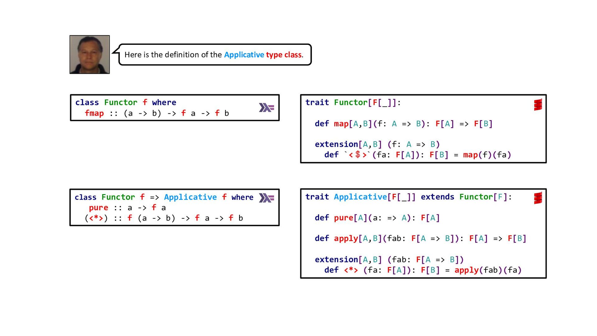
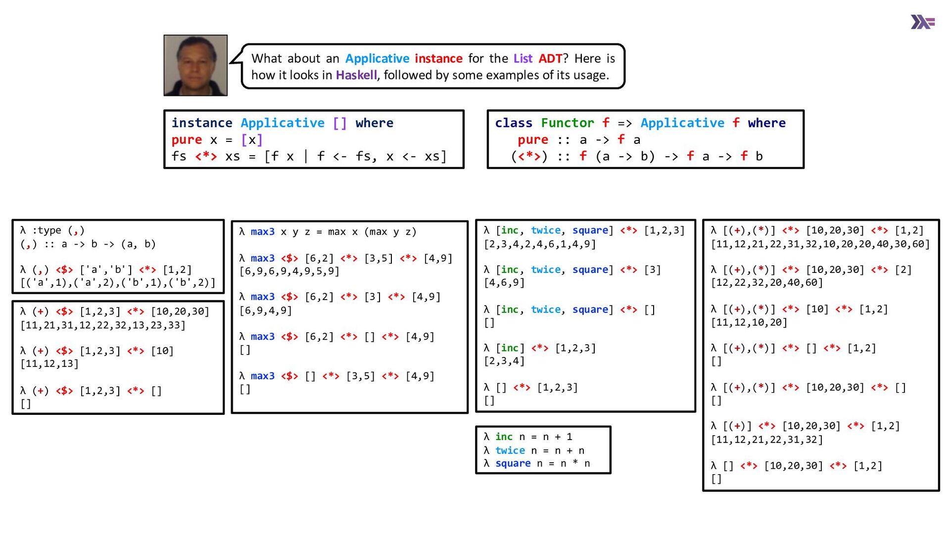
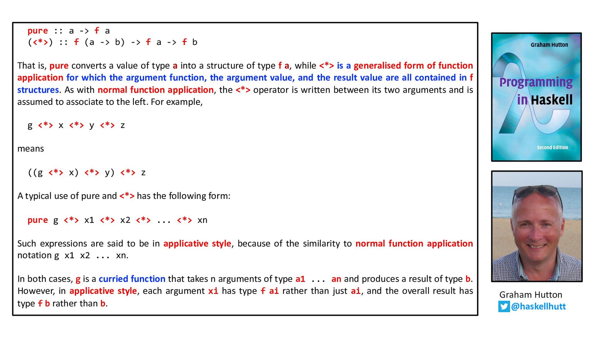
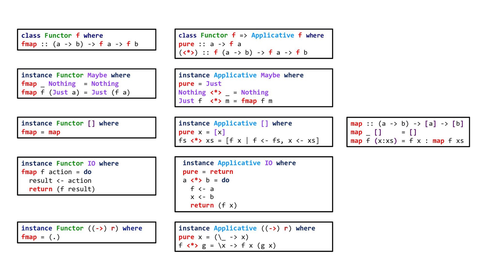
is how it looks in Haskell, followed by some examples of its usage. instance Applicative [] where pure x = [x] fs <*> xs = [f x | f <- fs, x <- xs] class Functor f => Applicative f where pure :: a -> f a (<*>) :: f (a -> b) -> f a -> f b λ (+) <$> [1,2,3] <*> [10,20,30] [11,21,31,12,22,32,13,23,33] λ (+) <$> [1,2,3] <*> [10] [11,12,13] λ (+) <$> [1,2,3] <*> [] [] λ max3 x y z = max x (max y z) λ max3 <$> [6,2] <*> [3,5] <*> [4,9] [6,9,6,9,4,9,5,9] λ max3 <$> [6,2] <*> [3] <*> [4,9] [6,9,4,9] λ max3 <$> [6,2] <*> [] <*> [4,9] [] λ max3 <$> [] <*> [3,5] <*> [4,9] [] λ inc n = n + 1 λ twice n = n + n λ square n = n * n λ [inc, twice, square] <*> [1,2,3] [2,3,4,2,4,6,1,4,9] λ [inc, twice, square] <*> [3] [4,6,9] λ [inc, twice, square] <*> [] [] λ [inc] <*> [1,2,3] [2,3,4] λ [] <*> [1,2,3] [] λ :type (,) (,) :: a -> b -> (a, b) λ (,) <$> ['a','b'] <*> [1,2] [('a',1),('a',2),('b',1),('b',2)] λ [(+),(*)] <*> [10,20,30] <*> [1,2] [11,12,21,22,31,32,10,20,20,40,30,60] λ [(+),(*)] <*> [10,20,30] <*> [2] [12,22,32,20,40,60] λ [(+),(*)] <*> [10] <*> [1,2] [11,12,10,20] λ [(+),(*)] <*> [] <*> [1,2] [] λ [(+),(*)] <*> [10,20,30] <*> [] [] λ [(+)] <*> [10,20,30] <*> [1,2] [11,12,21,22,31,32] λ [] <*> [10,20,30] <*> [1,2] []

So what does the Scala implementation of the Applicative instance
for the List ADT look like? instance Applicative [] where pure x = [x] fs <*> xs = [f x | f <- fs, x <- xs] Implementing pure in Scala is trivial: def pure[A](a: => A): List[A] = Cons(a, Nil) As for <*>, the above definition uses a list comprehension, firstly to extract function f from the list which is its first parameter, and secondly to extract the function’s argument x from the list which is its second parameter. It then applies f to x and returns a singleton list containing the result. How do we do the equivalent in Scala, where there is no list comprehension? For type constructors that are Monads, i.e. they have both a map method and a flatMap method, Scala provides for comprehensions. E.g. if we were implementing the List Monad, we would be able to implement Applicative’s apply method as follows: override def apply[A,B](fab: List[A => B]): List[A] => List[B] = fa => for { f <- fab a <- fa } yield f(a) But since in our particular case we are implementing the List Applicative rather than the List Monad, we have to find another way of implementing the apply method. enum List[+A]: case Cons(head: A, tail: List[A]) case Nil

If we define an append function for List, then we
can define the apply function recursively as follows: override def apply[A,B](fab: List[A => B]): List[A] => List[B] = fa => (fab, fa) match case (Nil, _) => Nil case (Cons(f,Nil), Nil) => Nil case (Cons(f,Nil), Cons(a,as)) => Cons(f(a),apply(fab)(as)) case (Cons(f,fs), fa) => append( apply(Cons(f, Nil))(fa), apply(fs)(fa)) object List: def append[A](lhs: List[A], rhs: List[A]): List[A] = foldRight((h: A,t: List[A]) => Cons(h,t))(rhs)(lhs) def foldRight[A,B](f: (A, B) => B)(b: B)(as: List[A]): B = as match case Nil => b case Cons(h,t) => f(h,foldRight(f)(b)(t)) Let’s define append in terms of the ubiquitous foldRight function: We can also use foldRight to implement the map function: def map[A, B](f: A => B): List[A] => List[B] = fa => foldRight((h:A,t:List[B]) => Cons(f(h),t))(Nil)(fa) See the next slide for the final code for this approach to the List Applicative, including a small test example.

trait Functor[F[_]]: def map[A,B](f: A => B): F[A] => F[B]
extension[A,B] (f: A => B) def `<＄>`(fa: F[A]): F[B] = map(f)(fa) trait Applicative[F[_]] extends Functor[F]: def pure[A](a: => A): F[A] def apply[A,B](fab: F[A => B]): F[A] => F[B] extension[A,B] (fab: F[A => B]) def <*> (fa: F[A]): F[B] = apply(fab)(fa) object List: def append[A](lhs: List[A], rhs: List[A]): List[A] = foldRight((h: A,t: List[A]) => Cons(h,t))(rhs)(lhs) def foldRight[A,B](f: (A, B) => B)(b: B)(as: List[A]): B = as match case Nil => b case Cons(h,t) => f(h,foldRight(f)(b)(t)) def of[A](as: A*): List[A] = as match case Seq() => Nil case _ => Cons(as.head, of(as.tail: _*)) enum List[+A]: case Cons(head: A, tail: List[A]) case Nil given listApplicative: Applicative[List] with override def pure[A](a: => A): List[A] = Cons(a, Nil) override def map[A, B](f: A => B): List[A] => List[B] = fa => foldRight((h:A,t:List[B]) => Cons(f(h),t))(Nil)(fa) override def apply[A,B](fab: List[A => B]): List[A] => List[B] = fa => (fab, fa) match case (Nil, _) => Nil case (Cons(f,Nil), Nil) => Nil case (Cons(f,Nil), Cons(a,as)) => Cons(f(a),apply(fab)(as)) case (Cons(f,fs), fa) => append( apply(Cons(f, Nil))(fa), apply(fs)(fa)) val inc: Int => Int = x => x + 1 val twice: Int => Int = x => x + x val square: Int => Int = x => x * x assert( List.of(inc, twice, square) <*> List.of(1, 2, 3) == List.of(2, 3, 4, 2, 4, 6, 1, 4, 9) ) assert( List.of(inc, twice, square) <*> Nil == Nil ) assert( List.of(inc, twice, square) <*> List.of(3) == List.of(4,6,9) ) assert( List.of(inc) <*> List.of(1,2,3) == List.of(2,3,4) ) assert( Nil <*> List.of(1, 2, 3) == Nil ) assert( Nil <*> Nil == Nil ) List Applicative Each function in the first list gets applied to each argument in the second list. @philip_schwarz

Before we move on, I’d like to share another way
of implementing the List Applicative which is very neat, but which turns out to be cheating, in that it amounts to making the List a Monad. If we take the code on the previous slide, then all we have to do is give List a flatten function: def flatten[A](xss: List[List[A]]): List[A] = foldRight[List[A],List[A]](append)(Nil)(xss) We can now greatly simplify the apply function as follows: def apply[A,B](fab: List[A => B]): List[A] => List[B] = fa => flatten( map((f: A => B) => map(a => f(a))(fa))(fab)) Another interesting thing is that if we also give the Maybe Applicative a fold function, then we can give it a flatten function… enum Option[+A]: case Some(a: A) case None def fold[B](ifEmpty: B)(f: A => B): B = this match case Some(a) => f(a) case None => ifEmpty def apply[A,B](fab: Option[A => B]): Option[A] => Option[B] = fa => flatten( map((f: A => B) => map(a => f(a))(fa))(fab)) object Option: def flatten[A](ooa: Option[Option[A]]): Option[A] = ooa.fold(None)(identity) …which means we can define the apply function the same way we did for List. This is cheating, because giving List the functions pure, map and flatten, is equivalent to giving it functions pure and flatMap, i.e. making it a Monad. def map[A, B](f: A => B): Option[A] => Option[B] = fa => fa.fold(None)(a => Some(f(a))) By the way: if we did the above, we could also define map in terms of fold.

The next slide just shows the Scala code for the
List and Option Applicative instances after applying the approach described in the previous slide.

object List: def flatten[A](xss: List[List[A]]): List[A] = foldRight[List[A],List[A]](append)(Nil)(xss) def append[A](lhs:
List[A], rhs: List[A]): List[A] = foldRight((h: A,t: List[A]) => Cons(h,t))(rhs)(lhs) def foldRight[A,B](f: (A, B) => B)(b: B)(as: List[A]): B = as match case Nil => b case Cons(h,t) => f(h,foldRight(f)(b)(t)) enum List[+A]: case Cons(head: A, tail: List[A]) case Nil given listApplicative: Applicative[List] with override def pure[A](a: => A): List[A] = Cons(a, Nil) override def map[A, B](f: A => B): List[A] => List[B] = fa => foldRight((h:A,t:List[B]) => Cons(f(h),t))(Nil)(fa) override def apply[A,B](fab: List[A => B]): List[A] => List[B] = fa => flatten( map((f: A => B) => map(a => f(a))(fa))(fab)) object Option: def flatten[A](ooa: Option[Option[A]]): Option[A] = ooa.fold(None)(identity) enum Option[+A]: case Some(a: A) case None def fold[B](ifEmpty: B)(f: A => B): B = this match case Some(a) => f(a) case None => ifEmpty given optionApplicative: Applicative[Option] with override def pure[A](a: => A): Option[A] = Some(a) override def map[A, B](f: A => B): Option[A] => Option[B] = fa => fa.fold(None)(a => Some(f(a))) override def apply[A,B](fab: Option[A=>B]): Option[A] => Option[B] = fa => flatten( map((f: A => B) => map(a => f(a))(fa))(fab)) trait Functor[F[_]]: def map[A,B](f: A => B): F[A] => F[B] extension[A,B] (f: A => B) def `<＄>`(fa: F[A]): F[B] = map(f)(fa) trait Applicative[F[_]] extends Functor[F]: def pure[A](a: => A): F[A] def apply[A,B](fab: F[A => B]): F[A] => F[B] extension[A,B] (fab: F[A => B]) def <*> (fa: F[A]): F[B] = apply(fab)(fa)

In the next 3 slides we take a look at
the IO Applicative.

IO Is An Applicative Functor, Too Another instance of Applicative
that we’ve already encountered is IO. This is how the instance is implemented: instance Applicative IO where pure = return a <*> b = do f <- a x <- b return (f x) Since pure is all about putting a value in a minimal context that still holds the value as the result, it makes sense that pure is just return. return makes an I/O action that doesn’t do anything. It just yields some value as its result, without performing any I/O operations like printing to the terminal or reading from a file. If <*> were specialized for IO, it would have a type of (<*>) :: IO (a -> b) -> IO a -> IO b. In the case of IO, it takes the I/O action a, which yields a function, performs the function, and binds that function to f. Then it performs b and binds its result to x. Finally, it applies the function f to x and yields that as the result. We used do syntax to implement it here. (Remember that do syntax is about taking several I/O actions and gluing them into one.) With Maybe and [], we could think of <*> as simply extracting a function from its left parameter and then applying it over the right one. With IO, extracting is still in the game, but now we also have a notion of sequencing, because we’re taking two I/O actions and gluing them into one. We need to extract the function from the first I/O action, but to extract a result from an I/O action, it must be performed. Miran Lipovača

Consider this: myAction :: IO String myAction = do a
<- getLine b <- getLine return $ a ++ b This is an I/O action that will prompt the user for two lines and yield as its result those two lines concatenated. We achieved it by gluing together two getLine I/O actions and a return, because we wanted our new glued I/O action to hold the result of a ++ b. Another way of writing this is to use the applicative style: myAction :: IO String myAction = (++) <$> getLine <*> getLine λ pure (++) <*> getLine <*> getLine foo bar "foobar" λ (++) <$> getLine <*> getLine foo bar "foobar" Let’s try out the IO Applicative. λ :type getLine getLine :: IO String instance Applicative IO where pure = return a <*> b = do f <- a x <- b return (f x)

import cats._ import cats.implicits._ import cats.effect.IO extension (l: String) def
`(++)`(r: String): String = l ++ r extension[A,B,F[_]] (f: A => B) def `<＄>`(fa: F[A])(using functor: Functor[F]): F[B] = functor.map(fa)(f) def getLine(): IO[String] = IO.pure(scala.io.StdIn.readLine) @main def main = val action1: IO[String] = IO.pure(`(++)`) <*> getLine() <*> getLine() println(action1.unsafeRunSync) val action2: IO[String] = `(++)` `<＄>` getLine() <*> getLine() println(action2.unsafeRunSync) sbt run foo bar "foobar” abc def ”abcdef” Here we try out the IO Applicative in Scala using the Cats Effect IO Monad, which being a Monad, is also an Applicative Functor. IO Applicative @philip_schwarz

Now that we have looked at the Applicative instances for
Maybe, for lists, and for IO actions, let’s see how Graham Hutton describes applicative style and summarises the similarities and differences between the three types of programming supported by the applicative style for the three above instances of Applicative.

pure :: a -> f a (<*>) :: f (a
-> b) -> f a -> f b That is, pure converts a value of type a into a structure of type f a, while <*> is a generalised form of function application for which the argument function, the argument value, and the result value are all contained in f structures. As with normal function application, the <*> operator is written between its two arguments and is assumed to associate to the left. For example, g <*> x <*> y <*> z means ((g <*> x) <*> y) <*> z A typical use of pure and <*> has the following form: pure g <*> x1 <*> x2 <*> ... <*> xn Such expressions are said to be in applicative style, because of the similarity to normal function application notation g x1 x2 ... xn. In both cases, g is a curried function that takes n arguments of type a1 ... an and produces a result of type b. However, in applicative style, each argument xi has type f ai rather than just ai, and the overall result has type f b rather than b. Graham Hutton @haskellhutt

Graham Hutton @haskellhutt the applicative style for Maybe supports a
form of exceptional programming in which we can apply pure functions to arguments that may fail without the need to manage the propagation of failure ourselves, as this is taken care of automatically by the applicative machinery. … the applicative style for lists supports a form of non-deterministic programming in which we can apply pure functions to multi-valued arguments without the need to manage the selection of values or the propagation of failure, as this is taken care of by the applicative machinery. … the applicative style for IO supports a form of interactive programming in which we can apply pure functions to impure arguments without the need to manage the sequencing of actions or the extraction of result values, as this is taken care of automatically by the applicative machinery. … The common theme between the instances is that they all concern programming with effects. In each case, the applicative machinery provides an operator <*> that allows us to write programs in a familiar applicative style in which functions are applied to arguments, with one key difference: the arguments are no longer just plain values but may also have effects, such as the possibility of failure, having many ways to succeed, or performing input/output actions. In this manner, applicative functors can also be viewed as abstracting the idea of applying pure functions to effectful arguments, with the precise form of effects that are permitted depending on the nature of the underlying functor. The next slide is a diagram illustrating the above with an example

λ pure max3 <*> ["jam"] <*> ["jaw"] <*> ["jar"] ["jaw"]
λ pure max3 <*> getLine <*> getLine <*> getLine jam jaw jar "jaw" λ max3 "jam" "jaw" "jar" "jaw" λ pure max3 <*> Just "jam" <*> Just "jaw" <*> Just "jar" Just "jaw” normal function appliction generalised form of function application exceptional programming normal programming non-deterministic programming interactive programming apply a pure function to arguments that may fail without the need to manage the propagation of failure ourselves apply a pure function to multi- valued arguments without the need to manage the selection of values or the propagation of failure apply a pure function to impure arguments without the need to manage the sequencing of actions or the extraction of result values apply a pure function to arguments

λ max3 <$> ["jam"] <*> ["jaw"] <*> ["jar"] ["jaw"] λ
max3 <$> getLine <*> getLine <*> getLine jam jaw jar "jaw" λ max3 "jam" "jaw" "jar" "jaw" λ max3 <$> Just "jam" <*> Just "jaw" <*> Just "jar" Just "jaw” Same code as on the previous slide, but this time using infix map .operator <$> .

Now let’s turn to the Applicative instance for functions. In
the next two slides we look at how Miran Lipovača describes it. @philip_schwarz

Functions As Applicatives Another instance of Applicative is (->) r,
or functions. We don’t often use functions as applicatives, but the concept is still really interesting, so let’s take a look at how the function instance is implemented. instance Applicative ((->) r) where pure x = (\_ -> x) f <*> g = \x -> f x (g x) When we wrap a value into an applicative value with pure, the result it yields must be that value. A minimal default context still yields that value as a result. That’s why in the function instance implementation, pure takes a value and creates a function that ignores its parameter and always returns that value. The type for pure specialized for the (->) r instance is pure :: a -> (r -> a). ghci> (pure 3) "blah" 3 Because of currying, function application is left-associative, so we can omit the parentheses. ghci> pure 3 "blah" 3 The instance implementation for <*> is a bit cryptic, so let’s just take a look at how to use functions as applicative functors in the applicative style: ghci> :t (+) <$> (+3) <*> (*100) (+) <$> (+3) <*> (*100) :: (Num a) => a -> a Miran Lipovača

ghci> (+) <$> (+3) <*> (*100) $ 5 508 Calling
<*> with two applicative values results in an applicative value, so if we use it on two functions, we get back a function. So what goes on here? When we do (+) <$> (+3) <*> (*100), we’re making a function that will use + on the results of (+3) and (*100) and return that. With (+) <$> (+3) <*> (*100) $ 5, (+3) and (*100) are first applied to 5, resulting in 8 and 500. Then + is called with 8 and 500, resulting in 508. The following code is similar: ghci> (\x y z -> [x,y,z]) <$> (+3) <*> (*2) <*> (/2) $ 5 [8.0,10.0,2.5] We create a function that will call the function \x y z -> [x,y,z] with the eventual results from (+3), (*2) and (/2). The 5 is fed to each of the three functions, and then \x y z -> [x,y,z] is called with those results. Miran Lipovača

Just like when we looked at Miran’s Lipovača’s example of
using Functor’s <$> operator, I think that the use of partially applied functions like (*3) and (+100) could be making the examples on the previous slide slightly harder to understand, by adding some unnecessary complexity. So here is the first example again, but this time using single-argument functions twice and square. λ inc n = n + 1 λ twice n = n + n λ square n = n * n λ :type inc inc :: Num a => a -> a λ :type twice twice :: Num a => a -> a λ :type square square :: Num a => a -> a λ :type (+) <$> twice <*> square (+) <$> twice <*> square :: Num b => b -> b λ (+) <$> twice <*> square $ 5 35 λ ((+) <$> twice <*> square) 5 35 λ (((+) . twice) <*> square) 5 35 λ (((+) . twice) 5)(square 5) 35 λ ((+) . twice) 5 (square 5) 35 λ (+) (twice 5) (square 5) 35 The other example would look like this: list3 <$> inc <*> twice <*> square $ 5. Instead of working through that right now, we are going to first see how the functions <$>, pure and <*> relate to combinatory logic, and then come back to both examples and work through them by viewing the functions as combinators. This will make evaluating the expressions in the examples easier to understand. It will also be quite interesting.

It turns out that the three functions of the Applicative
instance for functions, i.e. fmap, pure and <*>, are known in combinatory logic as combinators. The first one is called B and can be defined in terms of the other two, which are called K and S, and which are also called standard combinators. See the next slide for a table summarising some key facts about the combinators mentioned on this slide. According to a fundamental theorem of Schönfinkel and Curry, the entire 𝝀-calculus can be recast in the theory of combinators, which has only one basic operation: application. Abstraction is represented in this theory with the aid of two distinguished combinators: S and K, which are called standard combinators. … The two standard combinators, S and K, are sufficient for eliminating all abstractions, i.e. all bound variables from every 𝝀-expression. A combinator is a 𝝀-expression in which there are no occurrences of free variables. For example, the identity function 𝜆𝑥. 𝑥 is a combinator and is usually referred to by the identifier I. Another example is the fixed-point combinator … which is defined by 𝐘 = 𝜆ℎ. ( 𝜆𝑥. ℎ 𝑥 𝑥 𝜆𝑥. ℎ 𝑥 𝑥 ). Two further examples are the cancellator K given by 𝜆𝑥. 𝜆𝑦. 𝑥, and the distributor S given by 𝜆𝑓. 𝜆𝑔. 𝜆𝑥. 𝑓 𝑥(𝑔 𝑥). (Incidentally, the names for these are K and S rather than C and D because they were invented by Germans.) Now, as we shall see, any 𝝀-expression E can be converted into an applicative expression, i.e. an expression built entirely from function applications, lambda abstractions thereby being absent. To achieve this we require at least the two combinators (functions) S and K to be included in the expression syntax as additional constants. In fact, the 𝛌-calculus and the combinatory logic defined on these combinators are equivalent … In our presentation we shall also use the identity combinator I, although it should be noted that it can be defined in terms of S and K using the identity I=SKK. … … Although the complexity of the combinatory logic expressions which use only the S, K and I combinators is unacceptably high for use as a viable implementation technique, certain sub-expressions structures have much simpler forms, which are equivalent… Moreover, a much larger number of expressions may be simplified similarly if we introduce two further primitive combinators into the fixed set, using corresponding new identities. The new combinators in question are called the compositor, denoted by B, and the permutator, denoted by C, and are defined in the 𝝀-calculus by 𝐁 = 𝜆𝑓. 𝜆𝑥. 𝜆𝑦. 𝑓 𝑥 𝑦 and 𝐂 = 𝜆𝑓. 𝜆𝑥. 𝜆𝑦. 𝑓 𝑦 𝑥.

Name (Curry) Name (Smullyan) Definition Haskell function Signature Alternative name
and Lambda function Name (Schönfinkel) Definition in terms of other combinators S Starling 𝑆 𝑓 𝑔 𝑥 = 𝑓 𝑥 (𝑔 𝑥) Applicative's (<*>) on functions (a -> b -> c) -> (a -> b) -> a -> c Distributor 𝜆𝑥. 𝑦. 𝑧. 𝑥 𝑧(𝑦 𝑧) S Verschmelzungsfunktion (amalgamation function) K Kestrel 𝐾 𝑥 𝑦 = 𝑥 const a -> b -> a Cancellator 𝜆𝑥. 𝑦. 𝑥 K Konstanzfunktion (constant function) I Identity Bird 𝐼 𝑥 = 𝑥 id a -> a Idiot 𝜆𝑥. 𝑥 I Identitätsfunktion (identity function) SKK B Bluebird 𝐵 𝑓 𝑔 𝑥 = 𝑓 𝑔 𝑥 . (b -> c) -> (a -> b) -> a -> c Compositor 𝜆𝑥. 𝑦. 𝑧. 𝑥(𝑦 𝑧) Z Zusammensetzungsfunktion (composition function) S(KS)K C Cardinal 𝐶 𝑓 𝑥 𝑦 = 𝑓 𝑦 𝑥 flip (a -> b -> c) -> b -> a -> c Permutator 𝜆𝑥. 𝑦. 𝑧. 𝑥 𝑧 𝑦 T Vertauschungsfunktion (exchange function) S(BBS)(KK) https://www.angelfire.com/tx4/cus/combinator/birds.html https://www.johndcook.com/blog/2014/02/06/schonfinkel-combinators/ http://hackage.haskell.org/package/data-aviary-0.4.0/docs/Data-Aviary-Birds.html To Mock a Mockingbird - Raymond Smullyan Functional Programming - Anthony J. Field, Peter G. Harrison Lambda Calculus, Combinators and Functional Programming – G. Revesz. Recursive Programming Techniques– W. H. Burge

The previous two slides described combinators S, K, I, B
and C. The ones that we are interested in are S, K, and B, because they are the following functions of the Applicative instance for functions: fmap, pure and <*>. instance Applicative ((->) r) where pure x = (\_ -> x) f <*> g = \x -> f x (g x) instance Functor ((->) r) where fmap = (.) 𝐵 𝑓 𝑔 𝑥 = 𝑓 𝑔 𝑥 (<$>) :: Functor f => (a -> b) -> f a -> f b (<$>) = fmap Starling Kestrel K Cancellator Bluebird B Compositor (<*>) pure fmap (<$>) class Functor f => Applicative f where pure :: a -> f a (<*>) :: f (a -> b) -> f a -> f b class Functor f where fmap :: (a -> b) -> f a -> f b 𝐾 𝑥 𝑦 = 𝑥 Distributor 𝑆 𝑓 𝑔 𝑥 = 𝑓 𝑥 (𝑔 𝑥) S

(+) <$> twice <*> square $ 5 (((+) <$> twice)
<*> square) 5 (s (b (+) twice) square) 5 (b (+) twice) 5 (square 5) (+)(twice 5) (square 5) (+) 10 25 35 pure (+) <*> twice <*> square $ 5 (((pure (+)) <*> twice) <*> square) 5 (s (s (k (+)) twice) square) 5 (s (k (+)) twice) 5 (square 5) (k (+)) 5 (twice 5) (square 5) (+) (twice 5) (square 5) (+) 10 25 35 list3 <$> inc <*> twice <*> square $ 5 (((list3 <$> inc) <*> twice) <*> square) $ 5 (s (s (b list3 inc) twice) square) 5 (s (b list3 inc) twice) 5 (square 5) (b list3 inc) 5 (twice 5) (square 5) list3 (inc 5) (twice 5) (square 5) list3 6 10 25 [6,10,25] (pure list3 <*> inc <*> twice <*> square) 5 ((((pure list3) <*> inc) <*> twice) <*> square) 5 s (s (s (k list3) inc) twice) square 5 (s (s (k list3) inc) twice) 5 (square 5) (s (k list3) inc) 5 (twice 5) (square 5) (k list3) 5 (inc 5) (twice 5) (square 5) list3 (inc 5) (twice 5) (square 5) list3 6 10 25 [6,10,25] -- Combinators -- B: compositor b f g x = f (g x) -- K: cancellator k x y = x -- S: distributor s f g x = f x (g x) list3 x y z = [x,y,z]

class Functor f => Applicative f where pure :: a
-> f a (<*>) :: f (a -> b) -> f a -> f b instance Applicative ((->) r) where pure x = (\_ -> x) f <*> g = \x -> f x (g x) So what does the Scala equivalent of the Haskell implementation of the Applicative instance for functions look like? instance Functor ((->) r) where fmap = (.) class Functor f where fmap :: (a -> b) -> f a -> f b trait Functor[F[_]]: def map[A,B](f: A => B): F[A] => F[B] extension[A,B] (f: A => B) def `<＄>`(fa: F[A]): F[B] = map(f)(fa) trait Applicative[F[_]] extends Functor[F]: def pure[A](a: => A): F[A] def apply[A,B](fab: F[A => B]): F[A] => F[B] extension[A,B] (fab: F[A => B]) def <*> (fa: F[A]): F[B] = apply(fab)(fa) given functionApplicative[D]: Applicative[[C] =>> D => C] with override def pure[A](a: => A): D => A = x => a override def map[A,B](f: A => B): (D => A) => (D => B) = g => f compose g override def apply[A,B](f: D => A => B): (D => A) => (D => B) = g => n => f(n)(g(n)) (<$>) :: (Functor f) => (a -> b) -> f a -> f b f <$> x = fmap f x Here it is

val inc: Int => Int = x => x +
1 val twice: Int => Int = x => x + x val square: Int => Int = x => x * x def list3[A]: A => A => A => List[A] = x => y => z => List(x,y,z) assert( (map(map(inc)(twice))(square))(3) == 19) assert( (inc `<＄>` twice `<＄>` square)(3) == 19) assert( (pure(`(+)`) <*> twice <*> square)(5) == 35) assert( (`(+)` `<＄>` twice <*> square)(5) == 35) assert( (pure(list3) <*> inc <*> twice <*> square)(5) == List(6,10,25) ) assert( (list3 `<＄>` inc <*> twice <*> square)(5) == List(6,10,25) ) And here are some Scala tests showing the Applicative for functions in action.

pure a -> (d -> a) fmap (a -> b)
-> (d -> a) -> (d -> b) (<*>) (d -> a -> b) -> (d -> a) -> (d -> b) pure (a: => A): D => A Map (f: A => B): (D => A) => (D => B) <*> (fab: D => A => B): (D => A) => (D => B) pure a -> f a fmap (a -> b) -> f a -> f b (<*>) f (a -> b) -> f a -> f b pure a -> Maybe a fmap (a -> b) -> Maybe a -> Maybe b (<*>) Maybe (a -> b) -> Maybe a -> Maybe b pure (a: => A) : F[A] Map (f: A => B) : F[A] => F[B] <*> (fab: F[A => B]): F[A] => F[B] Pure. (a: => A) : Option[A] Map (f: A => B) : Option[A] => Option[B] <*> (fab: Option[A => B]): Option[A] => Option[B] Maybe Applicative ((->) d) Applicative Option Applicative ([C] =>> D => C) Applicative f a ⟹ (d -> a) ∃(d) e.g. Int f a ⟹ Maybe a F[A] ⟹ Option[A] F[A] ⟹ D => A ∃(D) e.g. Int It can be a bit hard to visualise how a function type can instantiate the Applicative type class, so here is a diagram that helps you do that by contrasting the signatures of pure, fmap, and (<*>) in two Applicative instances, one for Maybe and one for functions. @philip_schwarz

Now that we are thoroughly familiar with the Applicative for
functions, it’s finally time to see, on the next slide, how the palindrome checker function, which inspired this slide deck, works.

(≡) :: Eq a => a -> a -> Bool
(≡) x y = x == y reverse :: [a] -> [a] (<*>) :: Applicative f => f (a -> b) -> f a -> f b (<*>) f g x = f x (g x) palindrome :: Eq a => [a] -> Bool palindrome = (≡) <*> reverse ((->) d) Applicative (<*>) :: (d -> a -> b) -> (d -> a) -> (d -> b) d = [Char] a = [Char] b = Bool (<*>) :: ([Char] -> [Char] -> Bool) -> ([Char] -> [Char]) -> ([Char] -> Bool) (≡) reverse palindrome λ palindrome "amanaplanacanalpanama” True palindrome "amanaplanacanalpanama" ((≡) <*> reverse) "amanaplanacanalpanama" (s (≡) reverse) "amanaplanacanalpanama" ((≡) "amanaplanacanalpanama") (reverse "amanaplanacanalpanama") ((≡) "amanaplanacanalpanama") "amanaplanacanalpanama" "amanaplanacanalpanama" ≡ "amanaplanacanalpanama" True -- S, the Distributor -- combinator, aka Starling s f g x = f x (g x)

We have already seen hand rolled Scala code for the
Applicative type class and the Applicative instance for functions. Here it is again, with some new additional code implementing and testing the palindrome checker function. Not how if we use the Cats library we only need a few imports to get the new code to work. def ≣[A] = ((_: A) == (_: A)).curried def reverse[A]: Seq[A] => Seq[A] = _.reverse def palindrome[A]: Seq[A] => Boolean = ≣ <*> reverse @main def main = assert( palindrome("amanaplanacanalpanama") ) assert( ! palindrome("abcabc") ) assert( palindrome(List(1,2,3,3,2,1)) ) assert( ! palindrome(List(1,2,3,1,2,3)) ) trait Functor[F[_]]: def map[A,B](f: A => B): F[A] => F[B] extension[A,B] (f: A => B) def `<＄>`(fa: F[A]): F[B] = map(f)(fa) trait Applicative[F[_]] extends Functor[F]: def pure[A](a: => A): F[A] def apply[A,B](fab: F[A => B]): F[A] => F[B] extension[A,B] (fab: F[A => B]) def <*> (fa: F[A]): F[B] = apply(fab)(fa) given functionApplicative[D]: Applicative[[C] =>> D => C] with override def pure[A](a: => A): D => A = x => a override def map[A,B](f: A => B): (D => A) => (D => B) = g => f compose g override def apply[A,B](f: D => A => B): (D => A) => (D => B) = g => n => f(n)(g(n)) import cats._ import cats.implicits._ import cats.Applicative Option 1 Hand rolled Applicative type class and implicit instance for functions. Option 2 Predefined Cats Applicative type class and predefined implicit instance for functions.

The next slide is the last one and it is
just a recap of the Applicative instances we have seen in this deck.

instance Applicative ((->) r) where pure x = (\_ ->
x) f <*> g = \x -> f x (g x) instance Applicative Maybe where pure = Just Nothing <*> _ = Nothing Just f <*> m = fmap f m instance Applicative [] where pure x = [x] fs <*> xs = [f x | f <- fs, x <- xs] instance Applicative IO where pure = return a <*> b = do f <- a x <- b return (f x) instance Functor ((->) r) where fmap = (.) instance Functor IO where fmap f action = do result <- action return (f result) instance Functor [] where fmap = map instance Functor Maybe where fmap _ Nothing = Nothing fmap f (Just a) = Just (f a) class Functor f where fmap :: (a -> b) -> f a -> f b class Functor f => Applicative f where pure :: a -> f a (<*>) :: f (a -> b) -> f a -> f b map :: (a -> b) -> [a] -> [b] map _ [] = [] map f (x:xs) = f x : map f xs

That’s all. I hope you found that useful. @philip_schwarz

Function Applicative for Great Good of Palindro...

Function Applicative for Great Good of Palindrome Checker Function

More Decks by Philip Schwarz

Other Decks in Programming

Featured

Transcript