$30 off During Our Annual Pro Sale. View Details »

Elizabeth Ramirez - Kalman Filters for non-rocket science

Elizabeth Ramirez - Kalman Filters for non-rocket science

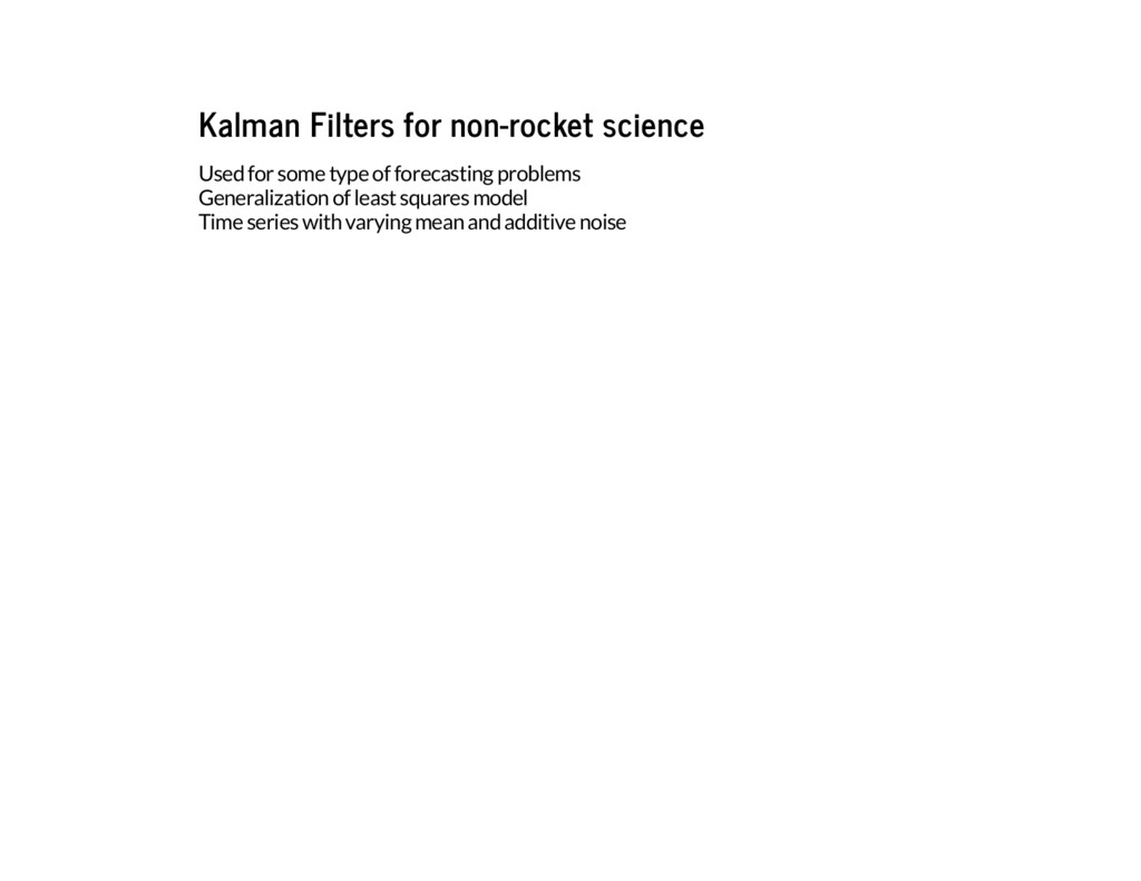
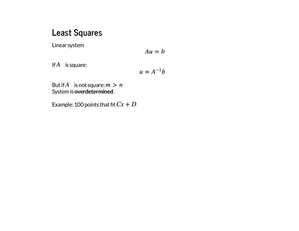
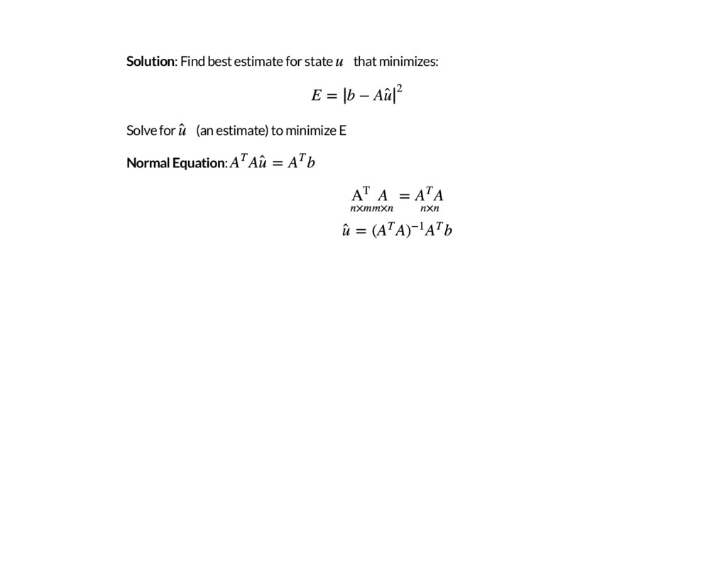
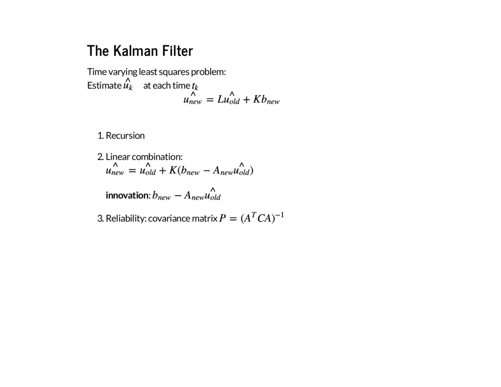
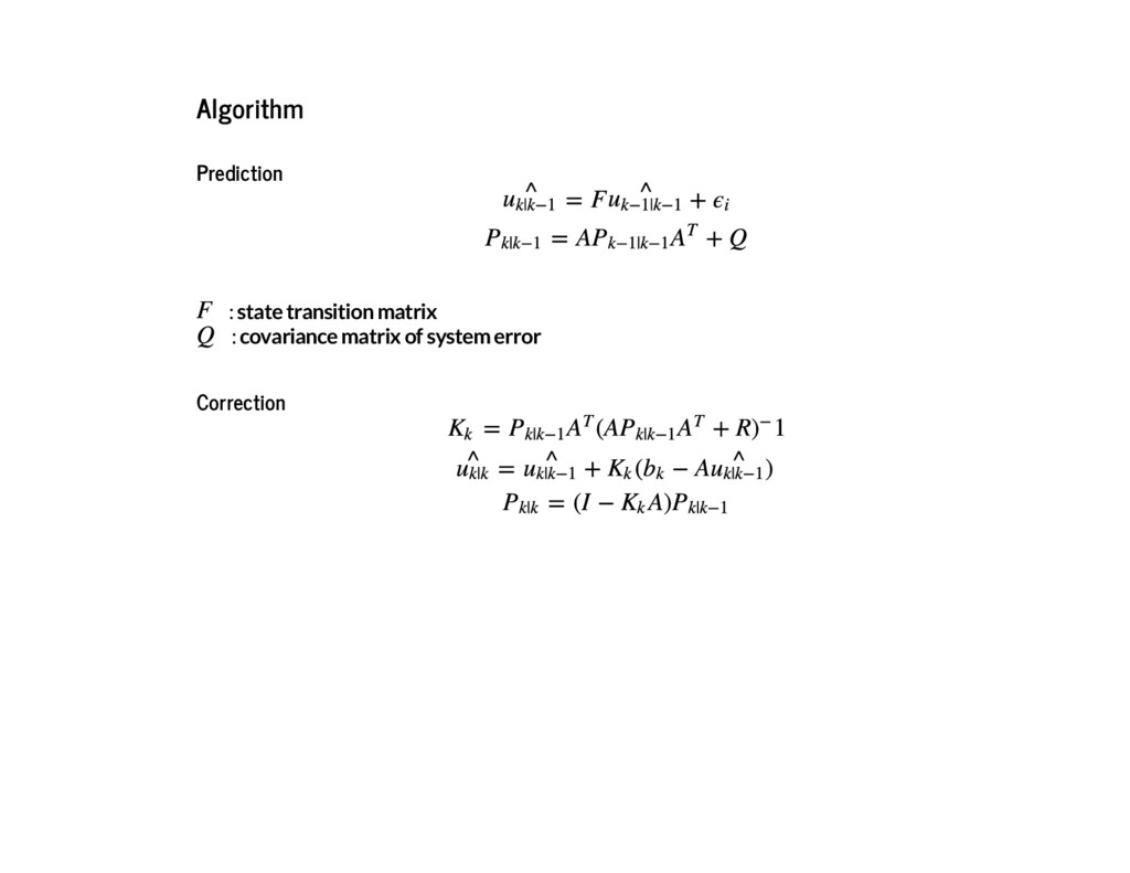
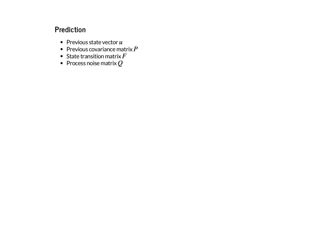
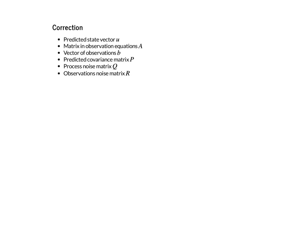
Kalman Filters have been widely used for scientific applications. No wonder people often think they involve complex math, however you can actually introduce the Kalman Filter in your daily data processing work, without the complex math you would imagine. This talk will show how to implement the discrete Kalman Filter in Python using NumPy and SciPy.

https://us.pycon.org/2016/schedule/presentation/2186/
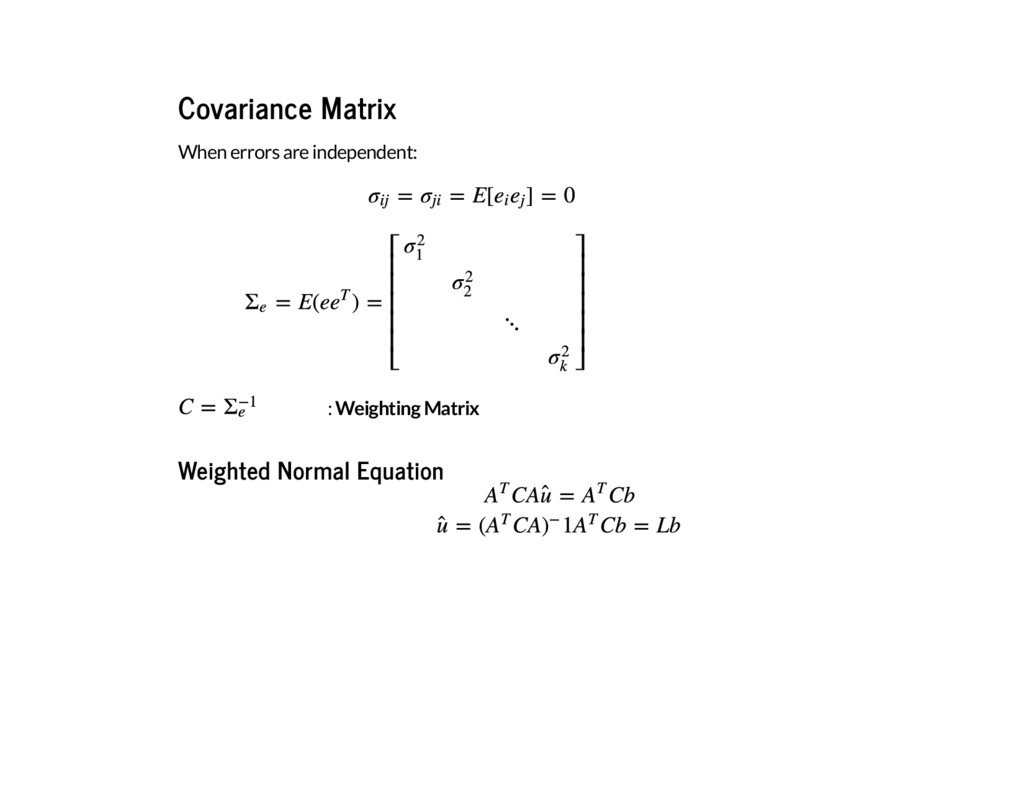
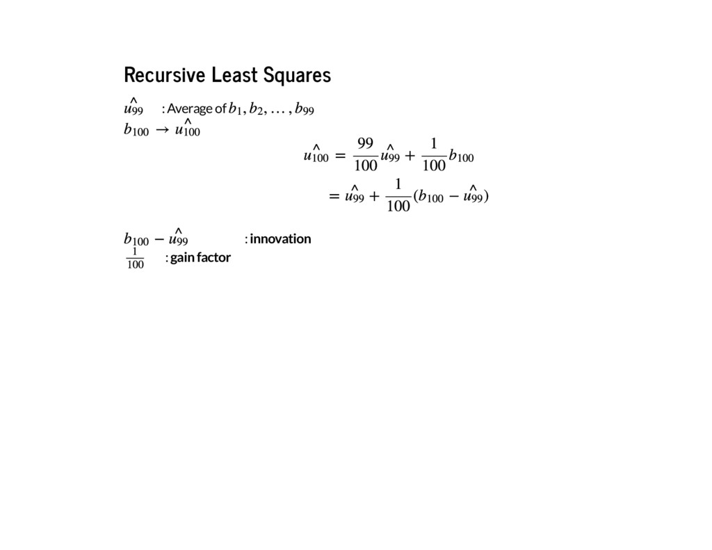
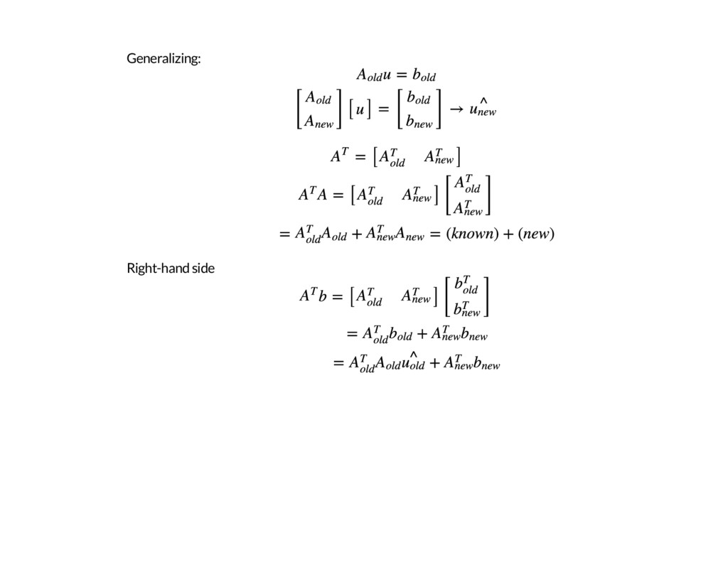
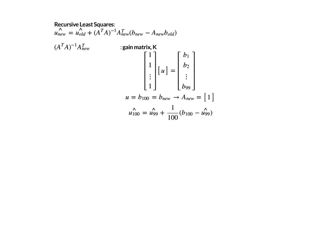
PyCon 2016

May 29, 2016
Tweet

More Decks by PyCon 2016

Other Decks in Programming

Transcript

  1. Kalman Filters for non-rocket science

    View Slide

  2. Background
    Named after named after Rudolf Kalman
    Original paper: [
    ]
    http://www.cs.unc.edu/~welch/kalman/media/pdf/Kalman1960.pdf
    (http://www.cs.unc.edu/~welch/kalman/media/pdf/Kalman1960.pdf)

    View Slide

  3. View Slide

  4. Kalman Filters for rocket science
    Used for Apollo Space Program of NASA in early 1960's
    Transcription of the original code available at [
    ]
    Implemented in AGC4 assembly language
    CCS: compare and skip
    TS: transfer to storage
    CA: clear and add
    http://www.ibiblio.org/apollo/
    (http://www.ibiblio.org/apollo/)

    View Slide

  5. View Slide

  6. Kalman Filters for non-rocket science
    Used for some type of forecasting problems
    Generalization of least squares model
    Time series with varying mean and additive noise

    View Slide

  7. Least Squares
    Linear system
    If is square:
    But if is not square:
    System is
    overdetermined
    .
    Example: 100 points that t

    View Slide

  8. Solution
    : Find best estimate for state that minimizes:
    Solve for (an estimate) to minimize E
    Normal Equation
    :

    View Slide

  9. Covariance Matrix
    When errors are independent:
    :
    Weighting Matrix
    Weighted Normal Equation

    View Slide

  10. Recursive Least Squares
    : Average of
    :
    innovation
    :
    gain factor

    View Slide

  11. Generalizing:
    Right-hand side

    View Slide

  12. Recursive Least Squares
    :
    :
    gain matrix, K

    View Slide

  13. The Kalman Filter
    Time varying least squares problem:
    Estimate at each time
    1. Recursion
    2. Linear combination:
    innovation
    :
    3. Reliability: covariance matrix

    View Slide

  14. Algorithm
    Prediction
    :
    state transition matrix
    :
    covariance matrix of system error
    Correction

    View Slide

  15. Implementation
    Output
    Predicted mean and covariance of the state (before the measurement)
    Estimated mean and covariance of the state (after the measurement)
    Innovation
    Filter gain

    View Slide

  16. Prediction
    Previous state vector
    Previous covariance matrix
    State transition matrix
    Process noise matrix

    View Slide

  17. In [29]: def predict(u, P, F, Q):
    u = numpy.dot(F, u)
    P = numpy.dot(F, numpy.dot(P, F.T)) + Q
    return u, P

    View Slide

  18. Correction
    Predicted state vector
    Matrix in observation equations
    Vector of observations
    Predicted covariance matrix
    Process noise matrix
    Observations noise matrix

    View Slide

  19. In [30]: def correct(u, A, b, P, Q, R):
    C = numpy.dot(A, numpy.dot(P, A.T)) + R
    K = numpy.dot(P, numpy.dot(A.T, numpy.linalg.inv(C)))
    u = u + numpy.dot(K, (b - numpy.dot(A, u)))
    P = P - numpy.dot(K, numpy.dot(C, K.T))
    return u, P

    View Slide

  20. In [124]: dt = 0.1
    A = numpy.array([[1, 0], [0, 1]])
    u = numpy.zeros((2, 1))
    # Random initial measurement centered at state value
    b = numpy.array([[u[0, 0] + randn(1)[0]], [u[1, 0] + randn(1)[0]]])
    P = numpy.diag((0.01, 0.01))
    F = numpy.array([[1.0, dt], [0.0, 1.0]])
    # Unit variance for the sake of simplicity
    Q = numpy.eye(u.shape[0])
    R = numpy.eye(b.shape[0])

    View Slide

  21. In [125]: N = 100
    predictions, corrections, measurements = [], [], []
    for k in numpy.arange(0, N):
    u, P = predict(u, P, F, Q)
    predictions.append(u)
    u, P = correct(u, A, b, P, Q, R)
    corrections.append(u)
    measurements.append(b)
    b = numpy.array([[u[0, 0] + randn(1)[0]],
    [u[1, 0] + randn(1)[0]]])
    print 'predicted final estimate: %f' % predictions[-1][0]
    print 'corrected final estimate: %f' % corrections[-1][0]
    print 'measured state: %f' % measurements[-1][0]
    predicted final estimate: -23.417806
    corrected final estimate: -22.995292
    measured state: -22.720059

    View Slide

  22. In [126]: t = numpy.arange(50, 100)
    fig = plt.figure(figsize=(15,15))
    axes = fig.add_subplot(2, 2, 1)
    axes.set_title("Kalman Filter")
    axes.plot(t, numpy.array(predictions)[50:100, 0], 'o', label='prediction')
    axes.plot(t, numpy.array(corrections)[50:100, 0], 'x', label='correction')
    axes.plot(t, numpy.array(measurements)[50:100, 0], '^', label='measurement')
    plt.legend()
    plt.show()

    View Slide

  23. Conclusions
    Kalman Filter is a viable forecasting technique for time series
    Computationally more ef cient
    Strang, Gilbert.
    Computational Science and Engineering

    View Slide

  24. Thank you!
    [email protected]
    @eramirem

    View Slide