Dimensionality reduction - squeezing out the good stuff with PCA by Aabir Abubaker Kar

Data is often high-dimensional - millions of pixels, frequencies, categories. A lot of this detail is unnecessary for data analysis - but how much exactly? This talk will discuss the ideas and techniques of dimensionality reduction, provide useful mathematical intuition about how it's done, and show you how Netflix uses it to lead you from binge to binge.

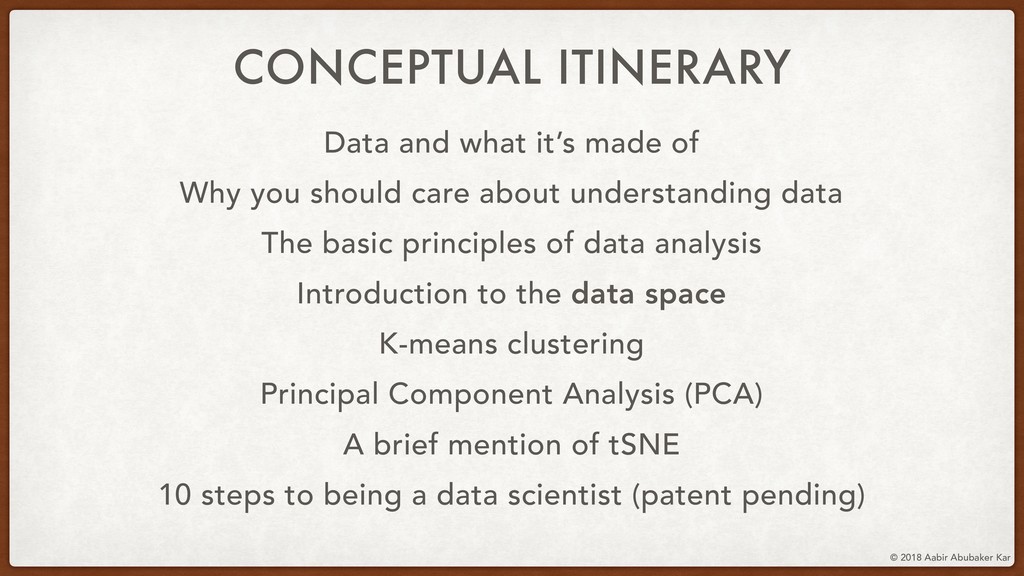
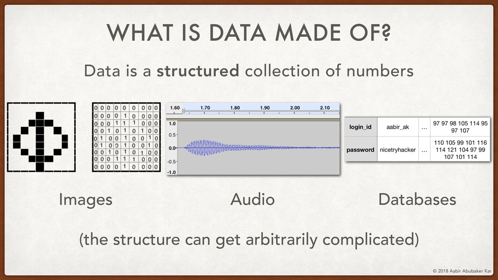
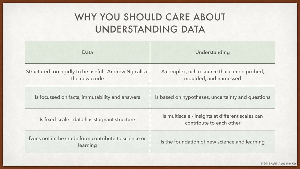
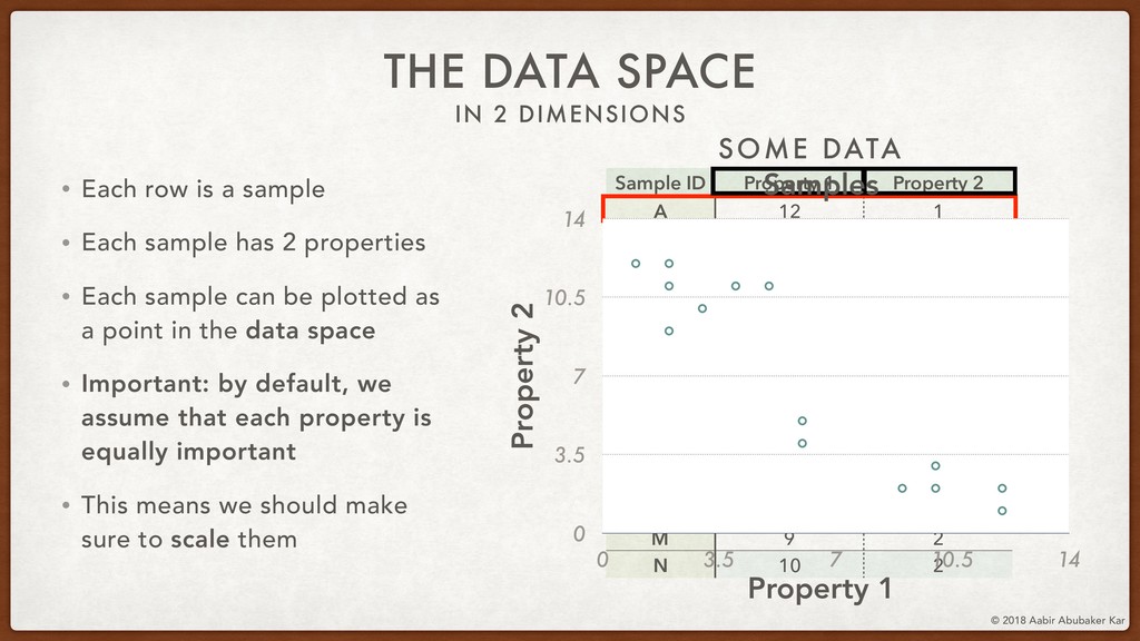
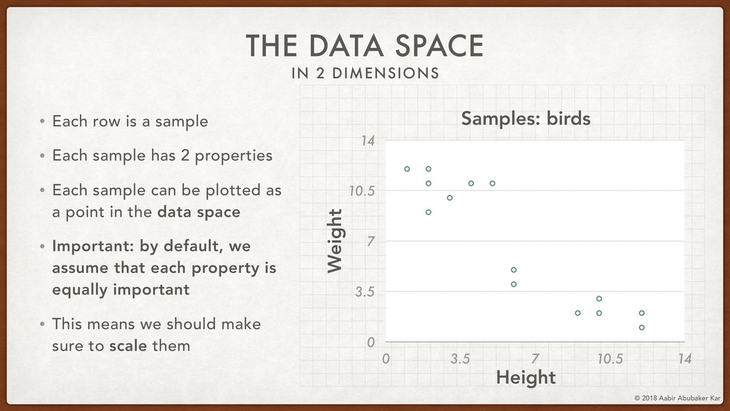
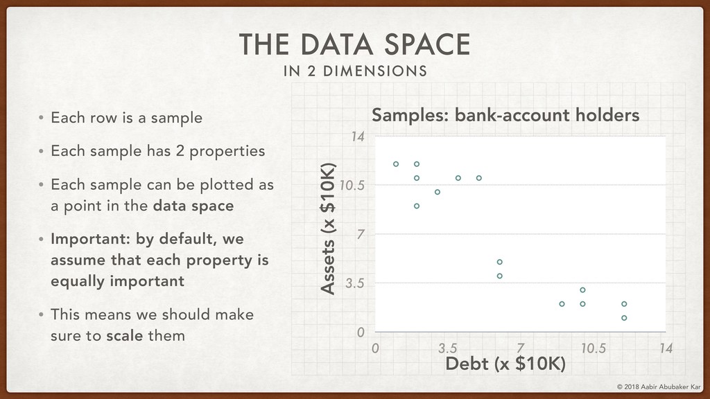
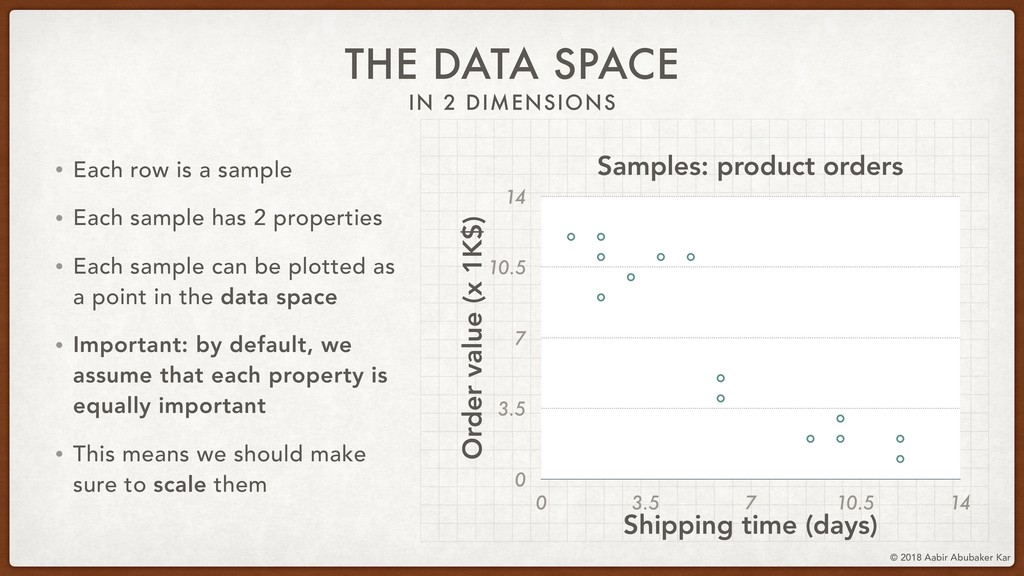
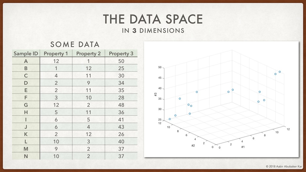
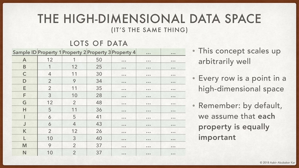
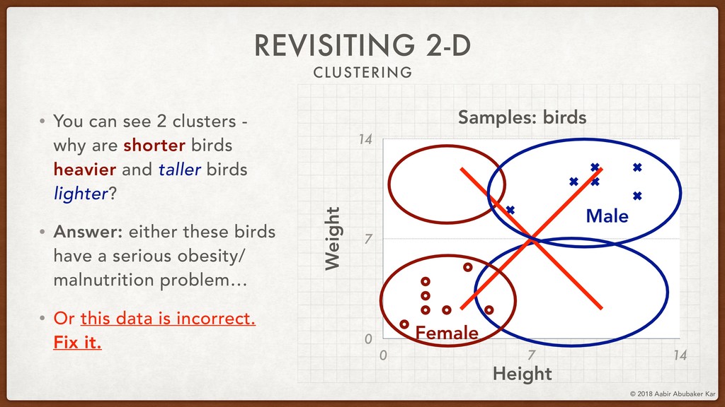
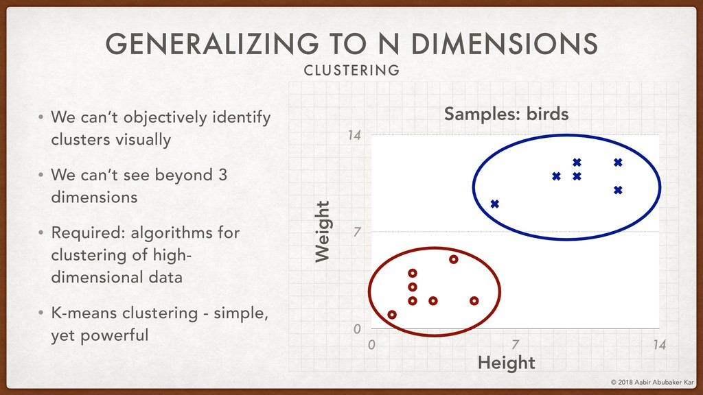
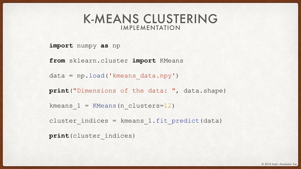
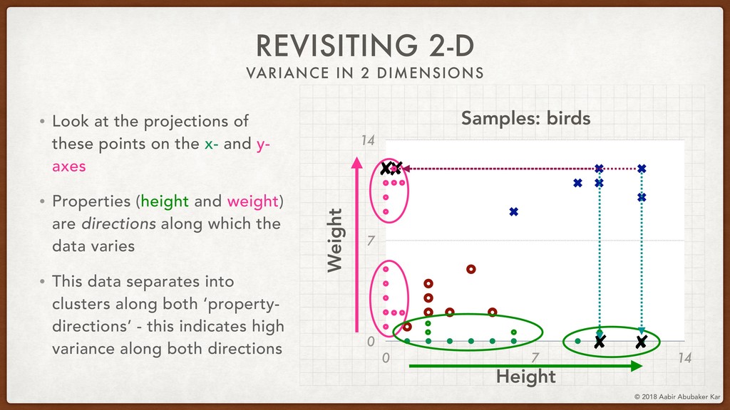
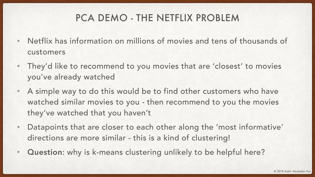
In this session, we'll start by remembering what data really is and what it stands for. Data is a structured set of numbers, and these numbers typically (hopefully!) hold some information. This will lead us naturally to the concept of a high-dimensional dataspace, the mystical realm in which data lives. It turns out that data in this space displays an extremely useful 'selection bias' - a datapoint can be known by the company it keeps. This is one of the basic ideas behind k-means clustering, which we will briefly discuss.

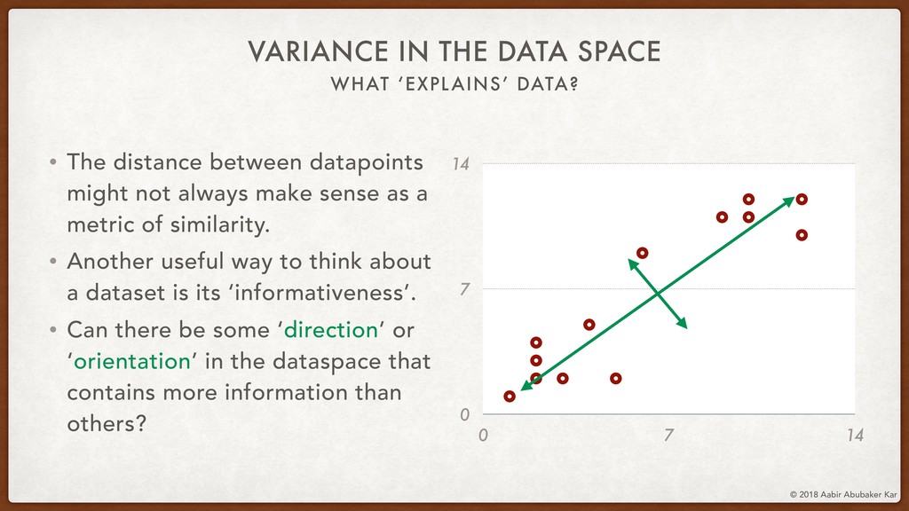
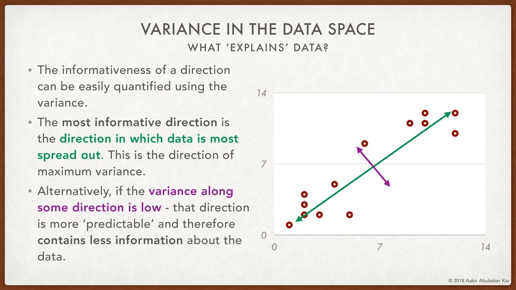
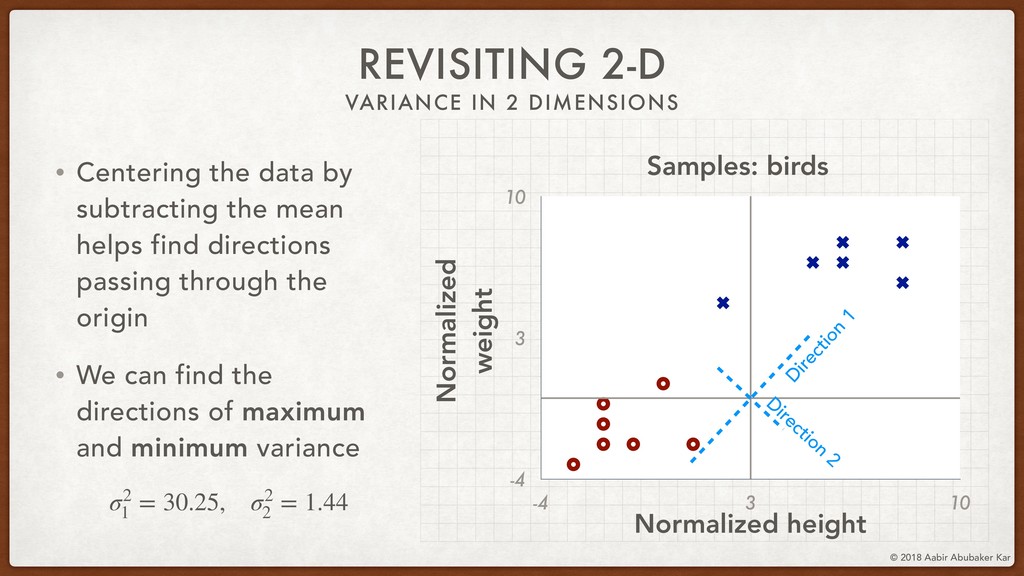
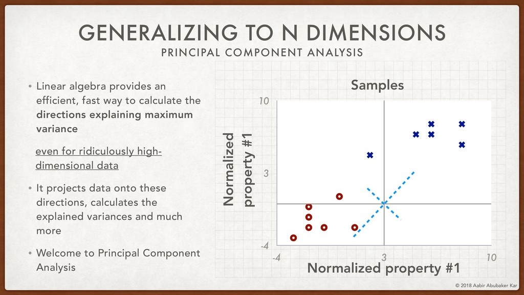
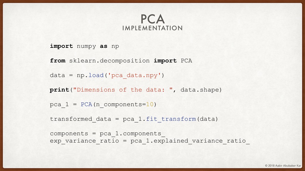
We'll then talk about the informative-ness of certain dimensions of the data space over others. This lays the mathematical foundation for the technique of Principal Component Analysis (PCA), which we will run on the Netflix movie dataset using scikit-learn.

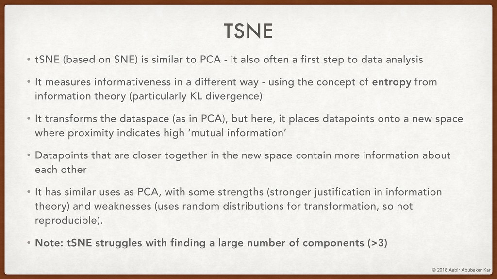
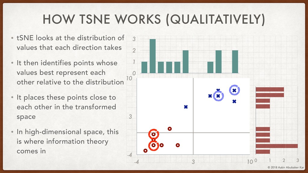
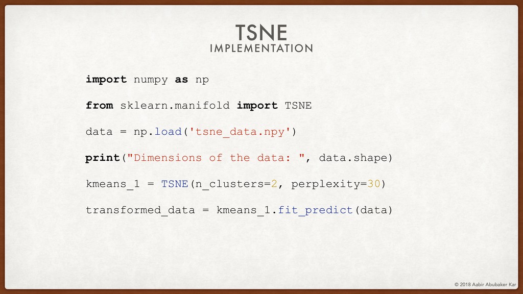
We will also touch upon tSNE, another popular dimensionality-reduction algorithms.

I will be using scikit-learn for processing and matplotlib for visualization. The purpose of this session is to introduce dimensionality-reduction to those who do not know it, and to provide useful guiding intuitions to those who do. We'll also discuss some seminal use-cases, with tips and warnings for your own applications.

Transcript

1. DIMENSIONALITY REDUCTION SQUEEZING OUT THE GOOD STUFF WITH PCA Aabir Abubaker Kar @aabir_ak
2. CONCEPTUAL ITINERARY Data and what it’s made of Why you should care about understanding data The basic principles of data analysis Introduction to the data space K-means clustering Principal Component Analysis (PCA) A brief mention of tSNE 10 steps to being a data scientist (patent pending) © 2018 Aabir Abubaker Kar
3. WHAT IS DATA MADE OF? Data is a structured collection of numbers Images Audio Databases (the structure can get arbitrarily complicated) © 2018 Aabir Abubaker Kar
4. WHY YOU SHOULD CARE ABOUT UNDERSTANDING DATA Data Understanding Structured too rigidly to be useful - Andrew Ng calls it the new crude A complex, rich resource that can be probed, moulded, and harnessed Is focussed on facts, immutability and answers Is based on hypotheses, uncertainty and questions Is fixed-scale - data has stagnant structure Is multiscale - insights at different scales can contribute to each other Does not in the crude form contribute to science or learning Is the foundation of new science and learning © 2018 Aabir Abubaker Kar
5. THE BASIC PRINCIPLES OF DATA ANALYSIS A datapoint can be known by the company it keeps Most data will display patterns that are indicative of the meta- information we are searching for
 © 2018 Aabir Abubaker Kar
6. SOME DATA Sample ID Property 1 Property 2 A 12 1 B 1 12 C 4 11 D 2 9 E 2 11 F 3 10 G 12 2 H 5 11 I 6 5 J 6 4 K 2 12 L 10 3 M 9 2 N 10 2 THE DATA SPACE • Each row is a sample • Each sample has 2 properties • Each sample can be plotted as a point in the data space • Important: by default, we assume that each property is equally important • This means we should make sure to scale them IN 2 DIMENSIONS 0 3.5 7 10.5 14 0 3.5 7 10.5 14 Property 1 Property 2 Samples © 2018 Aabir Abubaker Kar
7. IN 2 DIMENSIONS THE DATA SPACE 0 3.5 7 10.5 14 0 3.5 7 10.5 14 Height Weight Samples: birds • Each row is a sample • Each sample has 2 properties • Each sample can be plotted as a point in the data space • Important: by default, we assume that each property is equally important • This means we should make sure to scale them © 2018 Aabir Abubaker Kar
8. IN 2 DIMENSIONS THE DATA SPACE 0 3.5 7 10.5 14 0 3.5 7 10.5 14 Debt (x $10K) Assets (x $10K) Samples: bank-account holders • Each row is a sample • Each sample has 2 properties • Each sample can be plotted as a point in the data space • Important: by default, we assume that each property is equally important • This means we should make sure to scale them © 2018 Aabir Abubaker Kar
9. Shipping time (days) IN 2 DIMENSIONS THE DATA SPACE 0 3.5 7 10.5 14 0 3.5 7 10.5 14 Order value (x 1K$) Samples: product orders • Each row is a sample • Each sample has 2 properties • Each sample can be plotted as a point in the data space • Important: by default, we assume that each property is equally important • This means we should make sure to scale them © 2018 Aabir Abubaker Kar
10. THE DATA SPACE IN 3 DIMENSIONS SOME DATA Sample ID Property 1 Property 2 Property 3 A 12 1 50 B 1 12 25 C 4 11 30 D 2 9 34 E 2 11 35 F 3 10 28 G 12 2 48 H 5 11 36 I 6 5 41 J 6 4 43 K 2 12 26 L 10 3 40 M 9 2 37 N 10 2 37 © 2018 Aabir Abubaker Kar
11. THE HIGH-DIMENSIONAL DATA SPACE (IT’S THE SAME THING) LOTS OF DATA Sample ID Property 1Property 2 Property 3Property 4 … … A 12 1 50 … … … B 1 12 25 … … … C 4 11 30 … … … D 2 9 34 … … … E 2 11 35 … … … F 3 10 28 … … … G 12 2 48 … … … H 5 11 36 … … … I 6 5 41 … … … J 6 4 43 … … … K 2 12 26 … … … L 10 3 40 … … … M 9 2 37 … … … N 10 2 37 … … … • This concept scales up arbitrarily well • Every row is a point in a high-dimensional space • Remember: by default, we assume that each property is equally important © 2018 Aabir Abubaker Kar
12. THE HIGH-DIMENSIONAL DATA SPACE (IT’S THE SAME THING) So you can’t picture the 100th dimension? © 2018 Aabir Abubaker Kar
13. 0 7 14 0 7 14 0 7 14 0 7 14 CLUSTERING REVISITING 2-D • You can see 2 clusters - why are shorter birds heavier and taller birds lighter? • Answer: either these birds have a serious obesity/ malnutrition problem… • Or this data is incorrect. Fix it. Height Weight Samples: birds Male Female © 2018 Aabir Abubaker Kar
14. 0 7 14 0 7 14 CLUSTERING GENERALIZING TO N DIMENSIONS • We can’t objectively identify clusters visually • We can’t see beyond 3 dimensions • Required: algorithms for clustering of high- dimensional data • K-means clustering - simple, yet powerful Height Weight Samples: birds © 2018 Aabir Abubaker Kar
15. K-MEANS CLUSTERING • Input: • N datapoints each in the d- dimensional space • k, the number of clusters to be found • Output: • a list containing the cluster index for each datapoint • How it works: • Iteratively finds the k clusters such that each point is closest to the centroid (high-dimensional average) of its cluster Credits: Andrey A. Shabalin, shabal.in © 2018 Aabir Abubaker Kar
16. K-MEANS CLUSTERING • Limitations: • Not reproducible
 as the algorithm might not converge and is sensitive to initialization • True clusters may be of unequal size or density
 and centroids don’t represent these differences well • True clusters may be non-spherical (say, boomerang shaped)
 and as centroids are computed on the ‘nearest neighbors’, they won’t converge • There may be outliers in the data
 so centroids get skewed (the average of 2, 3, 3, 100 is 27) • Applications: • Automatic loan approval • Customer behavior classification • Cancer diagnosis • Image classification (NNs do it better) • Student performance analysis © 2018 Aabir Abubaker Kar
17. K-MEANS CLUSTERING IMPLEMENTATION import numpy as np from sklearn.cluster import KMeans data = np.load('kmeans_data.npy') print("Dimensions of the data: ", data.shape) kmeans_1 = KMeans(n_clusters=12) cluster_indices = kmeans_1.fit_predict(data) print(cluster_indices) © 2018 Aabir Abubaker Kar
18. WHAT ‘EXPLAINS’ DATA? VARIANCE IN THE DATA SPACE • The distance between datapoints might not always make sense as a metric of similarity. • Another useful way to think about a dataset is its ‘informativeness’. • Can there be some ‘direction’ or ‘orientation’ in the dataspace that contains more information than others? 0 7 14 0 7 14 © 2018 Aabir Abubaker Kar
19. WHAT ‘EXPLAINS’ DATA? VARIANCE IN THE DATA SPACE • The informativeness of a direction can be easily quantified using the variance. • The most informative direction is the direction in which data is most spread out. This is the direction of maximum variance. • Alternatively, if the variance along some direction is low - that direction is more ‘predictable’ and therefore contains less information about the data. 0 7 14 0 7 14 © 2018 Aabir Abubaker Kar
20. 0 7 14 0 7 14 • Look at the projections of these points on the x- and y- axes • Properties (height and weight) are directions along which the data varies • This data separates into clusters along both ‘property- directions’ - this indicates high variance along both directions VARIANCE IN 2 DIMENSIONS REVISITING 2-D Height Samples: birds Weight © 2018 Aabir Abubaker Kar
21. 0 7 14 0 7 14 • Formally, we can find the variance for the properties height and weight • • REVISITING 2-D Height Samples: birds Weight σ2 x = 1 N N ∑ i=1 (x − ¯ x)2 σ2 height = 15.2, σ2 weight = 19.36 VARIANCE IN 2 DIMENSIONS © 2018 Aabir Abubaker Kar
22. 0 7 14 0 7 14 • In other words, we need both directions (properties) to capture the variability of our data • In n dimensions, this means we’d need n directions (all n properties) • But what if we didn’t? REVISITING 2-D Height Samples: birds Weight VARIANCE IN 2 DIMENSIONS © 2018 Aabir Abubaker Kar
23. 0 7 14 0 7 14 • Consider a hybrid ‘direction’ made of 2 units of height and 1 unit of weight • Project the points down onto this direction • Each point has a coordinate on this new direction • The variance of these projected values is: REVISITING 2-D Height Samples: birds Weight 2 1 σ2 2×height+1×weight = 27.04 VARIANCE IN 2 DIMENSIONS 11.6 units © 2018 Aabir Abubaker Kar
24. • The new direction ‘explains’ more of the data than either of the original directions (height and weight)
 
 • One way to see this is to cluster the newly projected data using only this direction • Just one coordinate now explains the same two clusters σ2 2×height+1×weight = 27.04 0 7 14 0 7 14 REVISITING 2-D Height Samples: birds Weight 2 1 VARIANCE IN 2 DIMENSIONS σ2 height = 15.2, σ2 weight = 19.36 © 2018 Aabir Abubaker Kar
25. -4 3 10 -4 3 10 • Centering the data by subtracting the mean helps find directions passing through the origin • We can find the directions of maximum and minimum variance REVISITING 2-D Samples: birds Normalized height Normalized weight σ2 1 = 30.25, σ2 2 = 1.44 D irection 1 D irection 2 VARIANCE IN 2 DIMENSIONS © 2018 Aabir Abubaker Kar
26. PRINCIPAL COMPONENT ANALYSIS GENERALIZING TO N DIMENSIONS • Linear algebra provides an efficient, fast way to calculate the directions explaining maximum variance even for ridiculously high- dimensional data • It projects data onto these directions, calculates the explained variances and much more • Welcome to Principal Component Analysis Samples -4 3 10 -4 3 10 Normalized property #1 Normalized property #1 © 2018 Aabir Abubaker Kar
27. • Input: • N datapoints each in a d-dimensional space • Optionally, d2, the number of new directions to be found • Output: • d2 new ‘directions’, in decreasing order of explained variance • the projections of the N datapoints along these new directions • How it works: • jargon alert it finds the eigenvectors of the covariance matrix PRINCIPAL COMPONENT ANALYSIS (PCA) © 2018 Aabir Abubaker Kar
28. • Limitations: • No guarantee that PCA is prioritizing the ‘true’ directions • Depends on the topology of the data • Requires smart ‘normalisation’ (each of original d dimensions should have similar magnitudes) • To some extent, is a black box • Applications: • Feature extraction • Behaviour classification • Data exploration • Preliminary processing for many applications PRINCIPAL COMPONENT ANALYSIS (PCA) © 2018 Aabir Abubaker Kar
29. PCA IMPLEMENTATION import numpy as np from sklearn.decomposition import PCA data = np.load('pca_data.npy') print("Dimensions of the data: ", data.shape) pca_1 = PCA(n_components=10) transformed_data = pca_1.fit_transform(data) components = pca_1.components_ exp_variance_ratio = pca_1.explained_variance_ratio_ © 2018 Aabir Abubaker Kar
30. PCA DEMO - THE NETFLIX PROBLEM • Netflix has information on millions of movies and tens of thousands of customers • They’d like to recommend to you movies that are ‘closest’ to movies you’ve already watched • A simple way to do this would be to find other customers who have watched similar movies to you - then recommend to you the movies they’ve watched that you haven’t • Datapoints that are closer to each other along the ‘most informative’ directions are more similar - this is a kind of clustering! • Question: why is k-means clustering unlikely to be helpful here? © 2018 Aabir Abubaker Kar
31. PCA DEMO - THE NETFLIX PROBLEM Do demo © 2018 Aabir Abubaker Kar
32. THE NETFLIX PROBLEM - WHAT’S THE STORY? © 2018 Aabir Abubaker Kar
33. • tSNE (based on SNE) is similar to PCA - it also often a first step to data analysis • It measures informativeness in a different way - using the concept of entropy from information theory (particularly KL divergence) • It transforms the dataspace (as in PCA), but here, it places datapoints onto a new space where proximity indicates high ‘mutual information’ • Datapoints that are closer together in the new space contain more information about each other • It has similar uses as PCA, with some strengths (stronger justification in information theory) and weaknesses (uses random distributions for transformation, so not reproducible). • Note: tSNE struggles with finding a large number of components (>3) TSNE © 2018 Aabir Abubaker Kar
34. • tSNE looks at the distribution of values that each direction takes • It then identifies points whose values best represent each other relative to the distribution • It places these points close to each other in the transformed space • In high-dimensional space, this is where information theory comes in HOW TSNE WORKS (QUALITATIVELY) -4 3 10 -4 3 10 0 1 2 3 0 1 2 3 © 2018 Aabir Abubaker Kar
35. TSNE IMPLEMENTATION import numpy as np from sklearn.manifold import TSNE data = np.load('tsne_data.npy') print("Dimensions of the data: ", data.shape) kmeans_1 = TSNE(n_clusters=2, perplexity=30) transformed_data = kmeans_1.fit_predict(data) © 2018 Aabir Abubaker Kar
36. 10 STEPS TO BEING A DATA SCIENTIST (PATENT PENDING) 1. from sklearn import * 2. Read the docs 3. Read the docs 4. Read the docs 5. Read the docs 6. Read the docs 7. Read the docs 8. Read the docs 9. Read the docs 10. Read the docs © 2018 Aabir Abubaker Kar
37. THANK YOU © ScienceCartoonsPlus.com, Sidney Harris