Flow-induced phase separation of active colloids is controlled by boundary conditions

My DAMTP BioLunch talk on 7 June 2018.

Link to Movies:
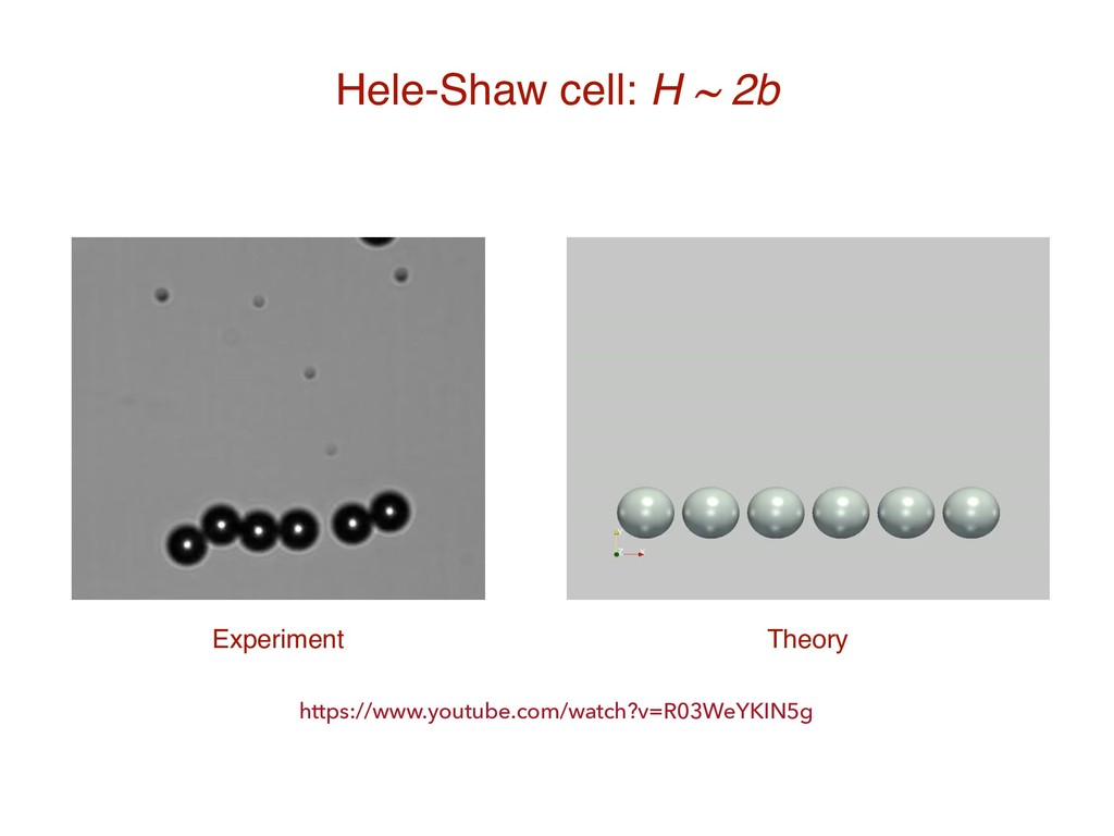
1. Slide-71 https://www.youtube.com/watch?v=R03WeYKIN5g
2. Slide-74 https://www.youtube.com/watch?v=Dq-SpTjvyNI
3. Slide-78 https://www.youtube.com/watch?v=FsiELGK15Y4
4. Slide-84 https://www.youtube.com/watch?v=LpAILGwD_JE
5. Slide-89 https://www.youtube.com/watch?v=2jUId3KUvNk

Abstract:
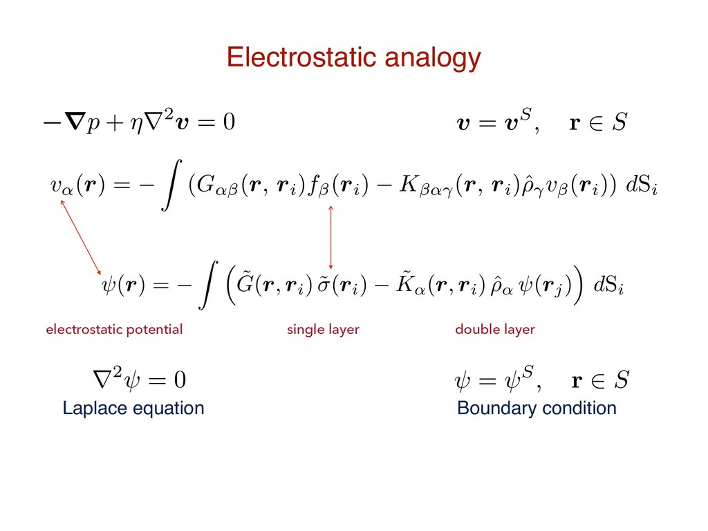
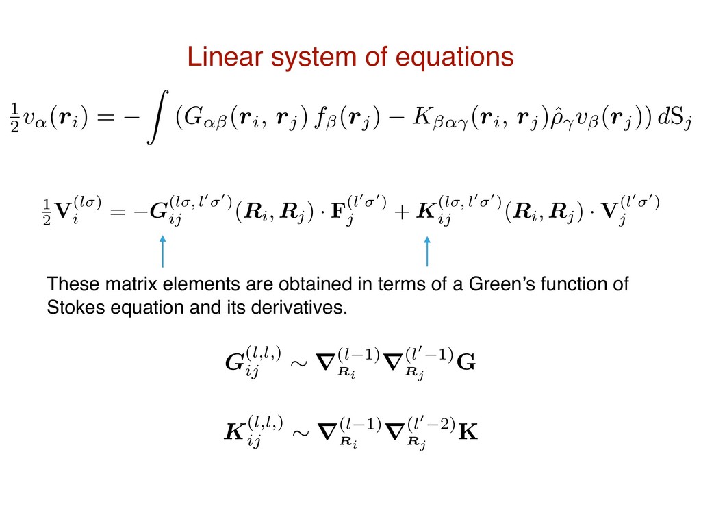
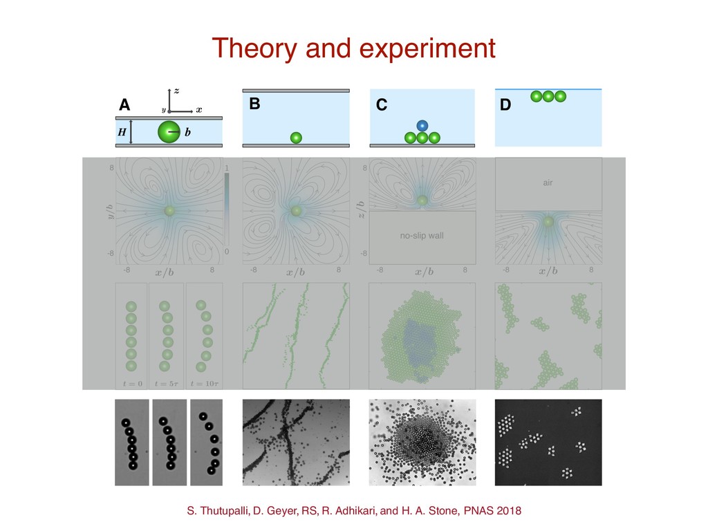
Active colloids - microorganisms, synthetic microswimmers, and self-propelling droplets - are known to self-organize into ordered structures at fluid-solid boundaries. Their mutual entrainment in the attractive component of the flow has been postulated as a possible mechanism underlying this phenomenon. In this talk, we describe this fluid-induced phase separation by combining experiments, theory, and numerical simulations, and demonstrate its control by changing the hydrodynamic boundary conditions. We show that, for flow in Hele-Shaw cells, metastable lines or stable traveling bands of colloids can be obtained by varying the cell height, while for flow bounded by a plane, dynamic crystallites are formed. At a plane no-slip wall, these crystallites are characterized by a continuous out-of-plane flux of particles that circulate and re-enter at the crystallite edges, thereby stabilizing them, while the crystallites are strictly two-dimensional at a plane where the tangential stress vanishes. These results are elucidated by deriving, using the boundary-domain integral formulation of Stokes flow, exact expressions for dissipative, long-ranged, many-body active forces and torques between them in respective boundary conditions.

Transcript

1. Flow-induced phase separation of active colloids is controlled by boundary conditions Reference: Shashi Thutupalli, Delphine Geyer, RS, R. Adhikari, H. A. Stone, PNAS 2018 Rajesh Singh DAMTP, University of Cambridge
2. Active colloids • Microorganisms Gollub lab, PRL 2010; Goldstein lab, PRL 2009 spontaneous symmetry breaking • Self-propelling droplets Thutupalli et al NJP 2011 self-propulsion by chemical asymmetry • Synthetic microswimmers Palacci et al Science 2013; Ebbens and Howse SM 2010
3. Active colloids • Microorganisms Gollub lab, PRL 2010; Goldstein lab, PRL 2009 spontaneous symmetry breaking • Self-propelling droplets Thutupalli et al NJP 2011 self-propulsion by chemical asymmetry • Synthetic microswimmers Palacci et al Science 2013; Ebbens and Howse SM 2010 non-equilibrium processes on the surface drive exterior fluid flow, even when the colloid is stationary the fluid stress may react back and cause self-propulsion in absence of external forces and torques fluid flow mediates long-range hydrodynamic interactions (HI) universal mechanisms due to the scale-separation for propulsion
4. Active colloids + Boundary condition Goldstein lab, PRL 2009
5. Active colloids + Boundary condition Goldstein lab, PRL 2009
6. S. Thutupalli, D. Geyer, RS, R. Adhikari, and H. A. Stone, PNAS 2018 Active colloids + Boundary conditions
7. S. Thutupalli, D. Geyer, RS, R. Adhikari, and H. A. Stone, PNAS 2018 Active colloids + Boundary conditions
8. S. Thutupalli, D. Geyer, RS, R. Adhikari, and H. A. Stone, PNAS 2018 Active colloids + Boundary conditions
9. S. Thutupalli, D. Geyer, RS, R. Adhikari, and H. A. Stone, PNAS 2018 Active colloids + Boundary conditions
10. S. Thutupalli, D. Geyer, RS, R. Adhikari, and H. A. Stone, PNAS 2018 Active colloids + Boundary conditions
11. Ideal active colloid A spherical colloid with slip boundary condition boundary velocity = rigid body motion + active slip v(ri) = Vi + ⌦i ⇥ ⇢i + vA i (⇢i )
12. Ideal active colloid Coordinate system for the ith sphere ri = Ri + ⇢i coordinate of the centre the radius vector point on the boundary
13. Ideal active colloid activity is represented by slip on a spherical surface slip is a mechanism to drive exterior flow without rigid body motion slip-induced flow may also cause self- propulsion without external forces flow is a unique function of slip and thus universal features are isolated problem reduced to obtaining force per unit area given the slip Coordinate system for the ith sphere ri = Ri + ⇢i coordinate of the centre the radius vector point on the boundary
14. Plan of the talk Boundary integral representation of Stokes flow
15. Plan of the talk Derivation of the force laws: Generalized Stokes laws Boundary integral representation of Stokes flow
16. Plan of the talk Derivation of the force laws: Generalized Stokes laws Covariant equations for the rigid body motion of active colloids Boundary integral representation of Stokes flow
17. Plan of the talk Derivation of the force laws: Generalized Stokes laws Covariant equations for the rigid body motion of active colloids Boundary integral representation of Stokes flow Active colloids at a plane surface Active colloids between parallel walls Active colloids near a plane wall Study dynamics of colloids in experimentally realizable settings
18. Equations of motion In microhydrodynamic regime, inertia is negligible Newton’s equations reduce to instantaneous balance of forces and torques Z fdSi + FP i = 0, Z ⇢i ⇥ fdSi + TP i = 0. surface force body force
19. Equations of motion In microhydrodynamic regime, inertia is negligible Newton’s equations reduce to instantaneous balance of forces and torques Z fdSi + FP i = 0, Z ⇢i ⇥ fdSi + TP i = 0. surface force body force , the force per unit area, is the normal component of the fluid stress. The fluid stress satisfies the Stokes equation r · v = 0, r · + ⇠ = 0, fluid velocity = pI + ⌘(rv + (rv)T ) r · v = 0, r · + ⇠ = 0, fluid stress active slip boundary condition v(ri) = Vi + ⌦i ⇥ ⇢i + vA i (⇢i ) f(ri) = ⇢i · (ri)
20. Equations of motion In microhydrodynamic regime, inertia is negligible Newton’s equations reduce to instantaneous balance of forces and torques Given the slip, we seek the force per unit area on the surface of colloids from the solution of above set of equations… Z fdSi + FP i = 0, Z ⇢i ⇥ fdSi + TP i = 0. surface force body force , the force per unit area, is the normal component of the fluid stress. The fluid stress satisfies the Stokes equation r · v = 0, r · + ⇠ = 0, fluid velocity = pI + ⌘(rv + (rv)T ) r · v = 0, r · + ⇠ = 0, fluid stress active slip boundary condition v(ri) = Vi + ⌦i ⇥ ⇢i + vA i (⇢i ) f(ri) = ⇢i · (ri)
21. Boundary integral representation Fluid velocity at any point in the bulk is given in terms of integrals on the surface of the colloids v↵(r) = Z (G↵ (r, ri)f (ri) K ↵ (r, ri)ˆ ⇢ v (ri)) dSi.
22. Boundary integral representation Fluid velocity at any point in the bulk is given in terms of integrals on the surface of the colloids Green’s function Stress tensor v↵(r) = Z (G↵ (r, ri)f (ri) K ↵ (r, ri)ˆ ⇢ v (ri)) dSi.
23. Boundary integral representation Fluid velocity at any point in the bulk is given in terms of integrals on the surface of the colloids Green’s function Stress tensor The integrand vanishes identically at any other boundary of the flow v↵(r) = Z (G↵ (r, ri)f (ri) K ↵ (r, ri)ˆ ⇢ v (ri)) dSi.
24. Boundary integral representation Fluid velocity at any point in the bulk is given in terms of integrals on the surface of the colloids Green’s function Stress tensor The integrand vanishes identically at any other boundary of the flow the Green’s function and the Stress tensor satisfy Stokes equation the integral admits analytical solution by Galerkin discretization for smooth boundaries like spheres problem reduced from the bulk three-dimensional flow to the two- dimensional surfaces of the colloids v↵(r) = Z (G↵ (r, ri)f (ri) K ↵ (r, ri)ˆ ⇢ v (ri)) dSi.
25. Electrostatic analogy v↵(r) = Z (G↵ (r, ri)f (ri) K ↵ (r, ri)ˆ ⇢ v (ri)) dSi. rp + ⌘r2v = 0 v = vS, r 2 S
26. Electrostatic analogy v↵(r) = Z (G↵ (r, ri)f (ri) K ↵ (r, ri)ˆ ⇢ v (ri)) dSi. rp + ⌘r2v = 0 (r) = Z ⇣ ˜ G(r, ri) ˜(ri) ˜ K↵(r, ri) ˆ ⇢↵ (rj) ⌘ dSi, electrostatic potential single layer double layer Laplace equation Boundary condition r2 = 0 = S, r 2 S v = vS, r 2 S
27. Galerkin expansion of the slip boundary velocity = rigid body motion + active slip v(ri) = Vi + ⌦i ⇥ ⇢i + vA i (⇢i )
28. Galerkin expansion of the slip boundary velocity = rigid body motion + active slip Expanding the slip in the basis of tensorial spherical harmonics Y(l) vA = 1 X l=1 1 (l 1)!(2l 3)!! V(l) · Y(l 1)(ˆ ⇢) v(ri) = Vi + ⌦i ⇥ ⇢i + vA i (⇢i )
29. Galerkin expansion of the slip boundary velocity = rigid body motion + active slip Expanding the slip in the basis of tensorial spherical harmonics Y(l) vA = 1 X l=1 1 (l 1)!(2l 3)!! V(l) · Y(l 1)(ˆ ⇢) Y(l) are dimensionless, symmetric, irreducible Cartesian tensors of rank l that form a complete, orthogonal basis on the sphere Y(l)(ˆ ⇢) = ( 1)l⇢l+1r(l)⇢ 1 v(ri) = Vi + ⌦i ⇥ ⇢i + vA i (⇢i )
30. Galerkin expansion of the slip boundary velocity = rigid body motion + active slip Expanding the slip in the basis of tensorial spherical harmonics Y(l) vA = 1 X l=1 1 (l 1)!(2l 3)!! V(l) · Y(l 1)(ˆ ⇢) Y(l) are dimensionless, symmetric, irreducible Cartesian tensors of rank l that form a complete, orthogonal basis on the sphere Y(l)(ˆ ⇢) = ( 1)l⇢l+1r(l)⇢ 1 v(ri) = Vi + ⌦i ⇥ ⇢i + vA i (⇢i ) Y (0) = 1, Y (1) ↵ = ˆ ⇢↵, Y (2) ↵ = ⇣ ˆ ⇢↵ ˆ ⇢ ↵ 3 ⌘ , Y (3) ↵ = ˆ ⇢↵ ˆ ⇢ ˆ ⇢ 1 5 [ˆ ⇢↵ + ˆ ⇢ ↵ + ˆ ⇢ ↵ ] .
31. vA ⇠ X V(l) · Y(l 1)
32. vA ⇠ X V(l) · Y(l 1)
33. vA ⇠ X V(l) · Y(l 1) V(l) = V(ls) + V(la) + V(lt) symmetric antisymmetric trace
34. l v(l )⇠ ( r(l 1)G ) 1 2 3 vA ⇠ X V(l) · Y(l 1) V(l) = V(ls) + V(la) + V(lt) symmetric antisymmetric trace
35. l v(l )⇠ ( r(l 1)G ) 1 2 3 Symmetric v(l )⇠ ( r(l 1)G )r(l 2)(r ⇥ G) vA ⇠ X V(l) · Y(l 1) V(l) = V(ls) + V(la) + V(lt) symmetric antisymmetric trace
36. l v(l )⇠ ( r(l 1)G ) 1 2 3 Symmetric v(l )⇠ ( r(l 1)G )r(l 2)(r ⇥ G) Antisymmetric ⇠ ( r(l 1)G )r(l 2)(r ⇥ G)( r(l 3)(r2G) ) vA ⇠ X V(l) · Y(l 1) V(l) = V(ls) + V(la) + V(lt) symmetric antisymmetric trace
37. l v(l )⇠ ( r(l 1)G ) 1 2 3 Symmetric v(l )⇠ ( r(l 1)G )r(l 2)(r ⇥ G) Antisymmetric ⇠ ( r(l 1)G )r(l 2)(r ⇥ G)( r(l 3)(r2G) ) Trace r(l 2)(r ⇥ G)( r(l 3)(r2G) ) vA ⇠ X V(l) · Y(l 1) V(l) = V(ls) + V(la) + V(lt) symmetric antisymmetric trace
38. l v(l )⇠ ( r(l 1)G ) 1 2 3 Symmetric v(l )⇠ ( r(l 1)G )r(l 2)(r ⇥ G) Antisymmetric ⇠ ( r(l 1)G )r(l 2)(r ⇥ G)( r(l 3)(r2G) ) Trace r(l 2)(r ⇥ G)( r(l 3)(r2G) ) vA ⇠ X V(l) · Y(l 1) in an unbounded domain of fluid flow v / r l, for slip V(l ) flow from the l-th mode has three independent terms: (a) symmetric irreducible gradients of G (b) its curl and, (c) its Laplacian V(l) = V(ls) + V(la) + V(lt) symmetric antisymmetric trace
39. Galerkin expansion of the traction We do a Galerkin expansion of boundary fields in the basis of the tensorial spherical harmonics f = 1 X l=1 2l 1 4⇡b2 F(l) i · Y(l 1)(ˆ ⇢) vA = 1 X l=1 1 (l 1)!(2l 3)!! V(l) · Y(l 1)(ˆ ⇢) The coefficients of the slip and traction are tensors of rank l and they can be written as a sum of three irreducible tensors of rank l, l-1 and l-2. The irreducible traction modes are represented by σ = s, symmetric, σ = a, antisymmetric, and σ = t trace of the tensor Given we seek explicit expression for F(l ) V(l ) F(l )
40. Linear system of equations 1 2 v↵(ri) = Z (G↵ (ri, rj) f (rj) K ↵ (ri, rj)ˆ ⇢ v (rj)) dSj f = 1 X l=1 2l 1 4⇡b2 F(l) i · Y(l 1)(ˆ ⇢) vA = 1 X l=1 1 (l 1)!(2l 3)!! V(l) · Y(l 1)(ˆ ⇢)
41. Linear system of equations 1 2 v↵(ri) = Z (G↵ (ri, rj) f (rj) K ↵ (ri, rj)ˆ ⇢ v (rj)) dSj f = 1 X l=1 2l 1 4⇡b2 F(l) i · Y(l 1)(ˆ ⇢) vA = 1 X l=1 1 (l 1)!(2l 3)!! V(l) · Y(l 1)(ˆ ⇢) 1 2 V(l ) i = G(l , l0 0) ij (Ri, Rj) · F(l0 0) j + K(l , l0 0) ij (Ri, Rj) · V(l0 0) j
42. Linear system of equations 1 2 v↵(ri) = Z (G↵ (ri, rj) f (rj) K ↵ (ri, rj)ˆ ⇢ v (rj)) dSj f = 1 X l=1 2l 1 4⇡b2 F(l) i · Y(l 1)(ˆ ⇢) vA = 1 X l=1 1 (l 1)!(2l 3)!! V(l) · Y(l 1)(ˆ ⇢) 1 2 V(l ) i = G(l , l0 0) ij (Ri, Rj) · F(l0 0) j + K(l , l0 0) ij (Ri, Rj) · V(l0 0) j These matrix elements are obtained in terms of a Green’s function of Stokes equation and its derivatives.
43. Linear system of equations 1 2 v↵(ri) = Z (G↵ (ri, rj) f (rj) K ↵ (ri, rj)ˆ ⇢ v (rj)) dSj 1 2 V(l ) i = G(l , l0 0) ij (Ri, Rj) · F(l0 0) j + K(l , l0 0) ij (Ri, Rj) · V(l0 0) j These matrix elements are obtained in terms of a Green’s function of Stokes equation and its derivatives.
44. Linear system of equations 1 2 v↵(ri) = Z (G↵ (ri, rj) f (rj) K ↵ (ri, rj)ˆ ⇢ v (rj)) dSj 1 2 V(l ) i = G(l , l0 0) ij (Ri, Rj) · F(l0 0) j + K(l , l0 0) ij (Ri, Rj) · V(l0 0) j These matrix elements are obtained in terms of a Green’s function of Stokes equation and its derivatives. G(l,l,) ij ⇠ r(l 1) Ri r(l0 1) Rj G K(l,l,) ij ⇠ r(l 1) Ri r(l0 2) Rj K
45. The coefficients of the traction are obtained from the solution the linear system of equations obtained from the Galerkin discretization of the boundary integrals Generalised Stokes laws F(l ) i = (l , 1s) ij · Vj (l , 2a) ij · ⌦j 1 X l0 0=1s (l , l0 0) ij · V(l0 0) j ,
46. The coefficients of the traction are obtained from the solution the linear system of equations obtained from the Galerkin discretization of the boundary integrals Generalised Stokes laws We call the above infinite set the generalized Stokes laws The generalised friction tensors relate the modes of slip and traction The expression for the generalised friction tensors is obtained in terms of a Green’s function of the Stokes equation The first two laws gives the force and torque on the colloids F(l ) i = (l , 1s) ij · Vj (l , 2a) ij · ⌦j 1 X l0 0=1s (l , l0 0) ij · V(l0 0) j ,
47. friction tensors for slip slip coefficients FH i = T T ij ·V i T R ij ·⌦ i 1 X l =1s (T, l ) ij · V(l ) j , TH i = RT ij ·V i RR ij ·⌦ i 1 X l =1s (R, l ) ij · V(l ) j . Active forces and torques The forces and torques depend on the positions of colloids through the friction tensors and orientations through the modes of the slip RS and Adhikari, PRL 2016
48. friction tensors for slip slip coefficients FH i = T T ij ·V i T R ij ·⌦ i 1 X l =1s (T, l ) ij · V(l ) j , TH i = RT ij ·V i RR ij ·⌦ i 1 X l =1s (R, l ) ij · V(l ) j . Active forces and torques The forces and torques depend on the positions of colloids through the friction tensors and orientations through the modes of the slip FH i + FP i + ˆ F i = 0, TH i + TP i + ˆ T i = 0. Body Brownian Hydrodynamic We use the above in Newton’s laws to obtain the rigid body motion RS and Adhikari, PRL 2016
49. Rigid body motion of active colloids T T ij ·Vj T R ij · ⌦j + FP i + ˆ Fi 1 X l =1s (T, l ) ij · V(l ) j = 0, RT ij ·Vj RR ij · ⌦j + TP i + ˆ Ti 1 X l =1s (R, l ) ij · V(l ) j = 0. RS and Adhikari, EJCM 2017, JPC 2018
50. Rigid body motion of active colloids T T ij ·Vj T R ij · ⌦j + FP i + ˆ Fi 1 X l =1s (T, l ) ij · V(l ) j = 0, RT ij ·Vj RR ij · ⌦j + TP i + ˆ Ti 1 X l =1s (R, l ) ij · V(l ) j = 0. Invert for rigid body motion RS and Adhikari, EJCM 2017, JPC 2018
51. Rigid body motion of active colloids T T ij ·Vj T R ij · ⌦j + FP i + ˆ Fi 1 X l =1s (T, l ) ij · V(l ) j = 0, RT ij ·Vj RR ij · ⌦j + TP i + ˆ Ti 1 X l =1s (R, l ) ij · V(l ) j = 0. Propulsion tensors relate modes of slip to rigid body motion White noises Mobility matrices connectors for forces and torques Vi = µT T ij · FP j + µT R ij · TP j + q 2kBTµT T ij · ⌘T j + q 2kBTµT R ij · ⇣R j + 1 X l =2s ⇡(T, l ) ij · V(l ) j + VA i ⌦i = µRT ij · FP j + µRR ij · TP j | {z } Passive + q 2kBTµRT ij · ⇣T j + q 2kBTµRR ij · ⌘R j | {z } Brownian + 1 X l =2s ⇡(R, l ) ij · V(l ) j + ⌦A i | {z } Active Invert for rigid body motion RS and Adhikari, EJCM 2017, JPC 2018
52. Rigid body motion of active colloids T T ij ·Vj T R ij · ⌦j + FP i + ˆ Fi 1 X l =1s (T, l ) ij · V(l ) j = 0, RT ij ·Vj RR ij · ⌦j + TP i + ˆ Ti 1 X l =1s (R, l ) ij · V(l ) j = 0. Propulsion tensors relate modes of slip to rigid body motion White noises Mobility matrices connectors for forces and torques Vi = µT T ij · FP j + µT R ij · TP j + q 2kBTµT T ij · ⌘T j + q 2kBTµT R ij · ⇣R j + 1 X l =2s ⇡(T, l ) ij · V(l ) j + VA i ⌦i = µRT ij · FP j + µRR ij · TP j | {z } Passive + q 2kBTµRT ij · ⇣T j + q 2kBTµRR ij · ⌘R j | {z } Brownian + 1 X l =2s ⇡(R, l ) ij · V(l ) j + ⌦A i | {z } Active ⇡(T, l ) ij = µT T ik · (T, l ) kj + µT R ik · (R, l ) kj , ⇡(R, l ) ij = µRT ik · (T, l ) kj + µRR ik · (R, l ) kj . Invert for rigid body motion RS and Adhikari, EJCM 2017, JPC 2018
53. Simulations ˙ Ri = Vi, ˙ pi = ⌦i ⇥ pi . ‣ Given a slip, the positions and orientations of the colloids are updated by integrating the following kinematic equations ‣ The boundary conditions in the bulk flow is implemented by choosing an appropriate Green’s function of Stokes equation ‣ The Steric repulsion between these finite size colloids is modelled using the truncated Lennard-Jones potential ‣ Problem reduced to the choice of a Green’s function and slip
54. Simulations ˙ Ri = Vi, ˙ pi = ⌦i ⇥ pi . ‣ Given a slip, the positions and orientations of the colloids are updated by integrating the following kinematic equations ‣ The boundary conditions in the bulk flow is implemented by choosing an appropriate Green’s function of Stokes equation ‣ The Steric repulsion between these finite size colloids is modelled using the truncated Lennard-Jones potential ‣ Problem reduced to the choice of a Green’s function and slip https://github.com/rajeshrinet/PyStokes
55. Theory and experiment S. Thutupalli, D. Geyer, RS, R. Adhikari, and H. A. Stone, PNAS 2018
56. Slip truncation vA i (⇢i ) = VA i + 1 15 V(3t) i · Y(2)(⇢i ) + V(2s) i · Y(1)(⇢i ) 1 75 V(4t) i · Y(3)(⇢i ). Truncate the slip expansion and choose coefficients which minimise the least-square deviation of the experimental and theoretical flow
57. Slip truncation vA i (⇢i ) = VA i + 1 15 V(3t) i · Y(2)(⇢i ) + V(2s) i · Y(1)(⇢i ) 1 75 V(4t) i · Y(3)(⇢i ). Truncate the slip expansion and choose coefficients which minimise the least-square deviation of the experimental and theoretical flow Experimental flow Theoretical flow
58. Green’s functions We derive expressions for the generalized friction tensors, mobility matrices, and propulsion tensors in terms of a Green’s function of Stokes equation. The Green’s function ensures that boundary conditions are satisfied in flow.
59. Green’s functions We derive expressions for the generalized friction tensors, mobility matrices, and propulsion tensors in terms of a Green’s function of Stokes equation. The Green’s function ensures that boundary conditions are satisfied in flow. Go ↵ = 1 8⇡⌘  ↵ r + r↵r r3 . Oseen tensor Plane free-slip surface: Blake-Aderogba tensor Gs ↵ (Ri, Rj) = Go ↵ (r) + ( ↵⇢ ↵⇢ 3 3 )G0 ↵ (r⇤).
60. Green’s functions We derive expressions for the generalized friction tensors, mobility matrices, and propulsion tensors in terms of a Green’s function of Stokes equation. The Green’s function ensures that boundary conditions are satisfied in flow. Plane no-slip wall: Gw ↵ (Ri, Rj) = Go ↵ (Ri Rj) + G⇤ ↵ (Ri, R⇤ j ), G⇤ ↵ = 1 8⇡⌘  ↵ r⇤ r⇤ ↵ r⇤ r⇤3 + 2h2 ✓ ↵⌫ r⇤3 3r↵r⌫ r⇤5 ◆ M⌫ 2h ✓ r⇤ 3 ↵⌫ + ⌫3r⇤ ↵ ↵3r⇤ ⌫ r⇤3 3r↵r⌫r⇤ 3 r⇤5 ◆ M⌫ . Lorentz-Blake tensor Go ↵ = 1 8⇡⌘  ↵ r + r↵r r3 . Oseen tensor Plane free-slip surface: Blake-Aderogba tensor Gs ↵ (Ri, Rj) = Go ↵ (r) + ( ↵⇢ ↵⇢ 3 3 )G0 ↵ (r⇤).
61. Green’s functions We derive expressions for the generalized friction tensors, mobility matrices, and propulsion tensors in terms of a Green’s function of Stokes equation. The Green’s function ensures that boundary conditions are satisfied in flow. Plane no-slip wall: Gw ↵ (Ri, Rj) = Go ↵ (Ri Rj) + G⇤ ↵ (Ri, R⇤ j ), G⇤ ↵ = 1 8⇡⌘  ↵ r⇤ r⇤ ↵ r⇤ r⇤3 + 2h2 ✓ ↵⌫ r⇤3 3r↵r⌫ r⇤5 ◆ M⌫ 2h ✓ r⇤ 3 ↵⌫ + ⌫3r⇤ ↵ ↵3r⇤ ⌫ r⇤3 3r↵r⌫r⇤ 3 r⇤5 ◆ M⌫ . Lorentz-Blake tensor Go ↵ = 1 8⇡⌘  ↵ r + r↵r r3 . Oseen tensor Plane free-slip surface: Blake-Aderogba tensor Gs ↵ (Ri, Rj) = Go ↵ (r) + ( ↵⇢ ↵⇢ 3 3 )G0 ↵ (r⇤). Parallel plane no-slip walls: G 2w ↵ (Ri, Rj) = 3hz(H z)(H h) ⇡⌘H3 ↵ 2r2 k r↵r r4 k ! , H ⇠ 2b, G 2w ↵ (Ri, Rj) = G o ↵ (rij) + G ⇤ ↵ (Ri, Rb⇤ j ) + G ⇤ ↵ (Ri, Rt⇤ j ) + G↵ , Liron-Mochon
62. Flow-induced phase separation
63. Hele-Shaw cell: H ~ 2b Experiment Theory https://www.youtube.com/watch?v=R03WeYKIN5g
64. Hele-Shaw cell: H ~ 2b Experiment Theory https://www.youtube.com/watch?v=R03WeYKIN5g
65. Hele-Shaw cell: H ~ 2b Experiment Theory https://www.youtube.com/watch?v=R03WeYKIN5g
66. Flow-induced phase separation
67. Hele-Shaw cell: H ~ 8b Experiment Theory https://www.youtube.com/watch?v=Dq-SpTjvyNI
68. Hele-Shaw cell: H ~ 8b Experiment Theory https://www.youtube.com/watch?v=Dq-SpTjvyNI
69. Hele-Shaw cell: H ~ 8b Experiment Theory https://www.youtube.com/watch?v=Dq-SpTjvyNI
70. Flow-induced phase separation
71. Plane no-slip wall Experiment Theory https://www.youtube.com/watch?v=FsiELGK15Y4
72. Plane no-slip wall Experiment Theory https://www.youtube.com/watch?v=FsiELGK15Y4
73. Plane no-slip wall Experiment Theory https://www.youtube.com/watch?v=FsiELGK15Y4
74. Flow-induced phase separation
75. Plane interface with no tangential stress Experiment Theory https://www.youtube.com/watch?v=LpAILGwD_JE
76. Plane interface with no tangential stress Experiment Theory https://www.youtube.com/watch?v=LpAILGwD_JE
77. Plane interface with no tangential stress Experiment Theory https://www.youtube.com/watch?v=LpAILGwD_JE
78. Theory and experiment S. Thutupalli, D. Geyer, RS, R. Adhikari, and H. A. Stone, PNAS 2018
79. Analytical and numerics-friendly formalism to study fluid-mediated interactions between active colloids that does not need to resolve explicit fluid degrees of freedom. Collective steady-states in active colloidal suspension are obtained from the flow-induced phase separation (FIPS) mechanisms. FIPS mechanisms are of dynamical origin. They are obtained from the balance of forces and torques on the colloids. In general, boundary conditions in the flow modify the active forces and torques, and thus, determine the collective behaviour. Summary
80. Analytical and numerics-friendly formalism to study fluid-mediated interactions between active colloids that does not need to resolve explicit fluid degrees of freedom. Collective steady-states in active colloidal suspension are obtained from the flow-induced phase separation (FIPS) mechanisms. FIPS mechanisms are of dynamical origin. They are obtained from the balance of forces and torques on the colloids. In general, boundary conditions in the flow modify the active forces and torques, and thus, determine the collective behaviour. Summary Thank You !
81. https://www.youtube.com/watch?v=2jUId3KUvNk Post-credit scene
82. https://www.youtube.com/watch?v=2jUId3KUvNk Post-credit scene