Upgrade to Pro — share decks privately, control downloads, hide ads and more …

Many-body microhydrodynamics of colloidal particles with active boundary layers

Many-body microhydrodynamics of colloidal particles with active boundary layers

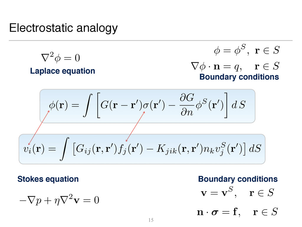
Colloidal particles with active boundary layers - regions surrounding the particles where nonequilibrium processes produce large velocity gradients - are common in many physical, chemical and biological contexts. The velocity or stress at the edge of the boundary layer determines the exterior fluid flow and, hence, the many-body interparticle hydrodynamic interaction. Here, we present a method to compute the many-body hydrodynamic interaction between $N$ spherical active particles induced by their exterior microhydrodynamic flow. First, we use a boundary integral representation of the Stokes equation to eliminate bulk fluid degrees of freedom. Then, we expand the boundary velocities and tractions of the integral representation in an infinite-dimensional basis of tensorial spherical harmonics and, on enforcing boundary conditions in a weak sense on the surface of each particle, obtain a system of linear algebraic equations for the unknown expansion coefficients. The truncation of the infinite series, fixed by the degree of accuracy required, yields a finite linear system that can be solved accurately and efficiently by iterative methods. The solution linearly relates the unknown rigid body motion to the known values of the expansion coefficients, motivating the introduction of propulsion matrices. These matrices completely characterize hydrodynamic interactions in active suspensions just as mobility matrices completely characterize hydrodynamic interactions in passive suspensions. The reduction in the dimensionality of the problem, from a three-dimensional partial differential equation to a two-dimensional integral equation, allows for dynamic simulations of hundreds of thousands of active particles on multi-core computational architectures. In our simulation of $10^4$ active colloidal particle in a harmonic trap, we find that the necessary and sufficient ingredients to obtain steady-state convective currents, the so-called “self- assembled pump”, are (a) one-body self-propulsion and (b) two-body rotation from the vorticity of the Stokeslet induced in the trap.

Rajesh Singh

July 11, 2015
Tweet

More Decks by Rajesh Singh

Other Decks in Research

Transcript

  1. Many-body microhydrodynamics of colloidal particles with active boundary layers Rajesh

    Singh, Somdeb Ghose and R. Adhikari The Institute of Mathematical Sciences Chennai, India
  2. 3 Microhydrodynamics of a single swimmer Non-equilibrium steady states of

    active particles in a harmonic potential Introduction Boundary integral equation Outline
  3. 5 Active matter Active matter describes systems driven out of

    equilibrium by constant consumption of energy, locally, to produce motion.
  4. 5 Active matter Active matter describes systems driven out of

    equilibrium by constant consumption of energy, locally, to produce motion. • Schools of fish • Flocks of birds
  5. 5 Active matter Active matter describes systems driven out of

    equilibrium by constant consumption of energy, locally, to produce motion. • Schools of fish • Flocks of birds J. Am. Chem. Soc., 2004, 126 (41), 13424–13431 • Catalytic motors
  6. 5 Active matter Active matter describes systems driven out of

    equilibrium by constant consumption of energy, locally, to produce motion. • Schools of fish • Flocks of birds J. Am. Chem. Soc., 2004, 126 (41), 13424–13431 • Catalytic motors • Microorganisms
  7. 5 Active matter Active matter describes systems driven out of

    equilibrium by constant consumption of energy, locally, to produce motion. • Schools of fish • Flocks of birds J. Am. Chem. Soc., 2004, 126 (41), 13424–13431 • Catalytic motors • Microorganisms The individual constituents of the assembly are called active particles.
  8. 6 Size Speed ⇠ cm ⇠ m ⇠ µm ⇠

    100µm Microhydrodynamics Scales in the system Features at this scale: • absence of inertia: counterintuitive • vanishing net-external force or torque • instantaneity of interactions • long range interactions
  9. 7 Microhydrodynamics: constraints M ˙ V = I · ndS

    + Fe I ˙ ⌦ = I r ⇥ · ndS + Te
  10. 7 Microhydrodynamics: constraints M ˙ V = I · ndS

    + Fe I ˙ ⌦ = I r ⇥ · ndS + Te absence of inertia
  11. 8 Microhydrodynamics: constraints M ˙ V = I · ndS

    + Fe I ˙ ⌦ = I r ⇥ · ndS + Te Force-free torque-free particles in absence of inertia
  12. 8 • Trivial solution: No motion in absence of external

    forces and torques • Non-trivial solutions describe the motion of an active particle. I · n dS = 0 I r ⇥ · n dS = 0 Microhydrodynamics: constraints M ˙ V = I · ndS + Fe I ˙ ⌦ = I r ⇥ · ndS + Te Force-free torque-free particles in absence of inertia
  13. Microhydrodynamics: momentum conservation • Boundary condition v = vS, r

    2 S n · = f, r 2 S Dirichlet Neumann • Stokes equation = pI + ⌘(rv + rvT ) r · = rp + ⌘r2v = 0 r · v = 0
  14. 10 Boundary layers vS = ✏⇣ 4⇡⌘ ES Interfacial double

    layer of surface charge and diffused counter-ions determine the vS slip = electrophoretic J. L. Anderson, Ann. Rev. Flu Mech 21(1989) Electrophoretic motion
  15. 11 Boundary layers Ciliary motion J. R. Blake JFM 46

    (1971) vS(r) = V + ⌦ ⇥ r + vc(r) slip = ciliary
  16. 11 Boundary layers Ciliary motion J. R. Blake JFM 46

    (1971) vS(r) = V + ⌦ ⇥ r + vc(r) slip = ciliary • as a spherical body with an active boundary layer • this leads to a slip velocity on the surface Ideal active particle
  17. 12 vS(r) = V + ⌦ ⇥ r + va(r)

    boundary velocity = rigid motion + active slip Ideal active particle
  18. 14 Boundary integral equation vi(r) = Z ⇥ Gij(r, r0)fj(r0)

    Kjik(r, r0)nkvS j (r0) ⇤ dS 8⇡⌘ Gij(r) = ij r + rirj r3 8⇡ Kijk(r) = 6 rirjrk r5
  19. 14 reduces a 3-dimensional problem of the solution of Stokes

    equation to a 2-dimensional integral equation on the boundary of the particles. massive simplification for computational purposes! Boundary integral equation vi(r) = Z ⇥ Gij(r, r0)fj(r0) Kjik(r, r0)nkvS j (r0) ⇤ dS 8⇡⌘ Gij(r) = ij r + rirj r3 8⇡ Kijk(r) = 6 rirjrk r5
  20. 15 r2 = 0 = S, r 2 S r

    · n = q, r 2 S Laplace equation Boundary conditions Electrostatic analogy (r) = Z  G(r r0) (r0) @G @n S(r0) d S
  21. 15 r2 = 0 = S, r 2 S r

    · n = q, r 2 S Laplace equation Boundary conditions Electrostatic analogy (r) = Z  G(r r0) (r0) @G @n S(r0) d S vi(r) = Z ⇥ Gij(r, r0)fj(r0) Kjik(r, r0)nkvS j (r0) ⇤ dS
  22. 15 Stokes equation Boundary conditions rp + ⌘r2v = 0

    v = vS, r 2 S n · = f, r 2 S r2 = 0 = S, r 2 S r · n = q, r 2 S Laplace equation Boundary conditions Electrostatic analogy (r) = Z  G(r r0) (r0) @G @n S(r0) d S vi(r) = Z ⇥ Gij(r, r0)fj(r0) Kjik(r, r0)nkvS j (r0) ⇤ dS
  23. 16 Electrostatic analogy (r) = Z  G(r r0) (r0)

    @G @n S(r0) d S vi(r) = Z ⇥ Gij(r, r0)fj(r0) Kjik(r, r0)nkvS j (r0) ⇤ dS
  24. 16 flow ~ potential traction ~ charge We can understand

    the microhydrodynamic phenomena guided by electrostatic analogies. The electrostatic equation is for scalar potential while the Stokes equation is for vector fields. Expect lots of indices in the formulation! Electrostatic analogy (r) = Z  G(r r0) (r0) @G @n S(r0) d S vi(r) = Z ⇥ Gij(r, r0)fj(r0) Kjik(r, r0)nkvS j (r0) ⇤ dS
  25. 18 • For discretisation of the integral equation, including both

    single and double layer, we expand the boundary fields in tensorial spherical harmonics Y(l). Tensorial spherical harmonics Y(l)
  26. 18 • For discretisation of the integral equation, including both

    single and double layer, we expand the boundary fields in tensorial spherical harmonics Y(l). Tensorial spherical harmonics Y(l) Y(l)(ˆ ⇢) = ( 1)l⇢l+1r(l) 1 ⇢ • Y(l) are symmetric traceless in all indices • Orthogonal basis function on sphere surface
  27. 18 • For discretisation of the integral equation, including both

    single and double layer, we expand the boundary fields in tensorial spherical harmonics Y(l). Tensorial spherical harmonics Y(l) Y(l)(ˆ ⇢) = ( 1)l⇢l+1r(l) 1 ⇢ • Y(l) are symmetric traceless in all indices • Orthogonal basis function on sphere surface • First three function in this basis are Y(0) = 1, Y(1) = ˆ ⇢, Y(2) = ✓ ˆ ⇢ˆ ⇢ 1 3 I ◆ .
  28. 19 Galerkin expansion of the boundary fields in Y(l) vi(r)

    = Z ⇥ Gij(r, r0)fj(r0) Kjik(r, r0)nkvS j (r0) ⇤ dS
  29. 19 Galerkin expansion of the boundary fields in Y(l) f(Rn

    + ⇢n ) = X 2l + 1 4⇡a2 F(l+1) n Y(l)( ˆ ⇢n ) v(Rn + ⇢n ) = X 1 l!(2l 1)!! V(l+1) n Y(l)( ˆ ⇢n ) Notation: implies a l-fold contraction between a tensor of rank l and a higher rank tensor vi(r) = Z ⇥ Gij(r, r0)fj(r0) Kjik(r, r0)nkvS j (r0) ⇤ dS
  30. 19 Galerkin expansion of the boundary fields in Y(l) f(Rn

    + ⇢n ) = X 2l + 1 4⇡a2 F(l+1) n Y(l)( ˆ ⇢n ) v(Rn + ⇢n ) = X 1 l!(2l 1)!! V(l+1) n Y(l)( ˆ ⇢n ) Notation: implies a l-fold contraction between a tensor of rank l and a higher rank tensor v(r) = P h G(l+1)(r, R) F(l+1) K(l+1)(r, R) V(l+1) i vi(r) = Z ⇥ Gij(r, r0)fj(r0) Kjik(r, r0)nkvS j (r0) ⇤ dS
  31. G(l+1)(r, R) = al ✓ 1 + a2 4l +

    6 r2 ◆ r(l)G(r, R) 20 Flow expression as derivatives of Green’s function v(r) = P h G(l+1)(r, R) F(l+1) K(l+1)(r, R) V(l+1) i
  32. G(l+1)(r, R) = al ✓ 1 + a2 4l +

    6 r2 ◆ r(l)G(r, R) 20 Flow expression as derivatives of Green’s function K(l+1)(r, R) = 4⇡al+1 (l 1)!(2l + 1)!! ✓ 1 + a2 4l + 6 r2 ◆ r(l 1)K(r, R) v(r) = P h G(l+1)(r, R) F(l+1) K(l+1)(r, R) V(l+1) i
  33. G(l+1)(r, R) = al ✓ 1 + a2 4l +

    6 r2 ◆ r(l)G(r, R) 20 Flow expression as derivatives of Green’s function • F(l+1) and V(l+1) are symmetric irreducible in their last l indices • This leads to systematic classification of the flow terms K(l+1)(r, R) = 4⇡al+1 (l 1)!(2l + 1)!! ✓ 1 + a2 4l + 6 r2 ◆ r(l 1)K(r, R) v(r) = P h G(l+1)(r, R) F(l+1) K(l+1)(r, R) V(l+1) i
  34. Irreducible part of the traction • Using angular momentum algebra,

    each F(l+1) and V(l+1) can be written as a sum of three irreducible tensors of rank (l − 1), l and (l + 1). • Each F(I) and V(l) can then be written as in terms of F(lσ) and V(lσ), which are individually symmetric irreducible tensors of rank l − σ.
  35. Irreducible part of the traction • Using angular momentum algebra,

    each F(l+1) and V(l+1) can be written as a sum of three irreducible tensors of rank (l − 1), l and (l + 1). • Each F(I) and V(l) can then be written as in terms of F(lσ) and V(lσ), which are individually symmetric irreducible tensors of rank l − σ. • Irreducible parts of the traction for l=0, 1 and 2 F(1) i = Fe i Monopole (3)
  36. Irreducible part of the traction • Using angular momentum algebra,

    each F(l+1) and V(l+1) can be written as a sum of three irreducible tensors of rank (l − 1), l and (l + 1). • Each F(I) and V(l) can then be written as in terms of F(lσ) and V(lσ), which are individually symmetric irreducible tensors of rank l − σ. • Irreducible parts of the traction for l=0, 1 and 2 F(1) i = Fe i Monopole (3) aF(2) ij = Sij + 1 2 ✏ijkTk Irreducible dipole (5) Anti-symmetric dipole (3)
  37. Irreducible part of the traction • Using angular momentum algebra,

    each F(l+1) and V(l+1) can be written as a sum of three irreducible tensors of rank (l − 1), l and (l + 1). • Each F(I) and V(l) can then be written as in terms of F(lσ) and V(lσ), which are individually symmetric irreducible tensors of rank l − σ. • Irreducible parts of the traction for l=0, 1 and 2 F(1) i = Fe i Monopole (3) aF(2) ij = Sij + 1 2 ✏ijkTk Irreducible dipole (5) Anti-symmetric dipole (3) a2F(3) ijk = ijk + 2 3 (2)✏ijl kl + 3 4 (2) ijDk Irreducible quadrupole (7) Antisymmetric quadrupole (5) Degenerate quadrupole (3)
  38. 22 Irreducible part of the velocity V(1) = V Va

    1 a V(2) = s + ✏ · (⌦ ⌦a) 1 a2 V3 = 2 3 (2) ✏ · + 3 5 (2) d Corresponding irreducible parts of the velocity
  39. 22 Irreducible part of the velocity V(1) = V Va

    1 a V(2) = s + ✏ · (⌦ ⌦a) 1 a2 V3 = 2 3 (2) ✏ · + 3 5 (2) d Corresponding irreducible parts of the velocity Va = hvai where the active translational velocity of the particle is and the active rotational velocity is ⌦a = 3 2a hˆ ⇢ ⇥ vai Here < - > indicates average over boundary.
  40. 23 Fluid flow at any order l has only three

    independent terms: irreducible gradient of the Green’s function, its curl and its Laplacian
  41. 23 Fluid flow at any order l has only three

    independent terms: irreducible gradient of the Green’s function, its curl and its Laplacian Fl = ✓ 1 + a2 4l + 6 r2 ◆ v(l ) = 0 = 1 = 2 l = 0 F0G · Q(10) — — l = 1 F1rG Q(20) 1 2 r ⇥ G · Q(21) — l = 2 F2rrG Q(30) 2 3 r r ⇥ G Q(31) 2 5 r2G Q(32) l = 3 F3rrrG Q(40) 3 4 rr · r ⇥ G Q(41) 36 35 rr2G Q(42) . . . . . . . . . . . . l Fl (l+1)r(l)G Q(l0) l l+1 (l) r(l) ⇥ G Q(l1) l(l+1) 2(2l+1) (l)r(l 2)r2G Q(l2)
  42. 31 One-body solution To determine velocity coefficients in terms of

    traction coefficients, expand the fluid velocity in the boundary integral equation and integrate on the surface of the particle
  43. 31 One-body solution To determine velocity coefficients in terms of

    traction coefficients, expand the fluid velocity in the boundary integral equation and integrate on the surface of the particle Rigid body motion of active particles including the active contributions, generalising Stokes law for one particle. V = Va + Fe 6⇡⌘a l=0 Va = hvai ⌦ = ⌦a + Te 8⇡⌘a3 l=1, antisymmetric ⌦a = 3 2a hˆ ⇢ ⇥ vai
  44. 32 Many-body solution The net flow is a superposition of

    flow due to each particle, because of linearity of the Stokes equation v = N X m=1 vm(r, Rm) The presence of n-th particle changes the boundary condition on m-th particle. And hence the traction and velocity boundary condition has to be satisfied simultaneously. This means a large systems of linear equations which must be solved simultaneously to obtain the irreducible coefficients and hence the RBM of the many active particles.
  45. 33 The formal solution for the rigid body motion of

    passive particles is written in terms of mobility matrices Many-body solution ⌦n = ⌦a n + X h µRT nm · Fe m + µRR nm · Te m + ⇡(R,l+1) nm · V(l+1) m i Vn = Va + X h µTT nm · Fe m + µTR nm · Te m + ⇡(T,l+1) nm · V(l+1) m i
  46. 34 The formal solution for the rigid body motion of

    active particles can then be written in terms of mobility and propulsion matrices Many-body solution ⌦n = ⌦a n + X h µRT nm · Fe m + µRR nm · Te m + ⇡(R,l+1) nm · V(l+1) m i Vn = Va + X h µTT nm · Fe m + µTR nm · Te m + ⇡(T,l+1) nm · V(l+1) m i
  47. ⌦n = ⌦a n + X h µRT nm ·

    Fe m + µRR nm · Te m + ⇡(R,l+1) nm · V(l+1) m i 35 The formal solution for the rigid body motion of active particles can then be written in terms of mobility and propulsion matrices Many-body solution Vn = Va + X h µTT nm · Fe m + µTR nm · Te m + ⇡(T,l+1) nm · V(l+1) m i The above clearly shows that particle can both rotate and translate in the absence of external forces and torques Rajesh Singh, Somdeb Ghose and R. Adhikari J. Stat. Mech. (2015)
  48. 36 Summary of the particulate theory Stokes equation Integral representation

    Galerkin expansion Sum of irreducible parts Classification of flow
  49. 36 Summary of the particulate theory Stokes equation Integral representation

    Galerkin expansion Sum of irreducible parts Classification of flow ⌦n = ⌦a n + X h µRT nm · Fe m + µRR nm · Te m + ⇡(R,l+1) nm · V(l+1) m i Vn = Va + X h µTT nm · Fe m + µTR nm · Te m + ⇡(T,l+1) nm · V(l+1) m i Eliminating unknowns
  50. 36 Summary of the particulate theory Stokes equation Integral representation

    Galerkin expansion Sum of irreducible parts Classification of flow • Generalisation of Stokes equation for active particles • Rigid body motion in terms of mobility and propulsion matrices • The infinitely many propulsion matrices, as compared to only four mobility matrices, account for the rich and diverse phenomena shown by active dynamical systems ⌦n = ⌦a n + X h µRT nm · Fe m + µRR nm · Te m + ⇡(R,l+1) nm · V(l+1) m i Vn = Va + X h µTT nm · Fe m + µTR nm · Te m + ⇡(T,l+1) nm · V(l+1) m i Eliminating unknowns
  51. Microswimming of C. Reinhardtii Flagella driven by dyenin motors J.

    S. Guasto, K. A. Johnson, J. P. Gollub, PRL (2010) Microhydrodynamic flow around C. Reinhardtii
  52. Microswimming of C. Reinhardtii Flagella driven by dyenin motors J.

    S. Guasto, K. A. Johnson, J. P. Gollub, PRL (2010) Microhydrodynamic flow around C. Reinhardtii
  53. Microswimming of C. Reinhardtii Flagella driven by dyenin motors J.

    S. Guasto, K. A. Johnson, J. P. Gollub, PRL (2010) Time-dependent flow field Microhydrodynamic flow around C. Reinhardtii
  54. 39 V ( t ) = V0 + V1 exp(

    iwt ) + V2 exp(2 iwt ) Fit the following experimental quantities • translational motion to fix the degenerate quadrupole. • location of the stagnation point from the center of the swimmer to fix the symmetric irreducible dipole and quadrupole Sum the contributions to the flow from these three modes and compare ... Microhydrodynamic flow around C. Reinhardtii 0 0.25 0.50 0.75 1.00 −0.2 0 0.2 0.4 0.6 0.8 t/T V(t) / Vmax v cm fit
  55. Experiment J. S. Guasto, K. A. Johnson, J. P. Gollub

    PRL (2010) Theory S. Ghose, R. Adhikari PRL (2014)
  56. 49 Lighthill (1952) and Blake (1971) considered a sphere with

    axisymmetric slip velocity vS ⇢ = ˆ ⇢ · vS = 0, vS = ˆ · vS = 0, vS ✓ = ˆ ✓ · vS = B1 sin ✓ + B2 sin ✓ cos ✓, Squirmer model
  57. 49 Lighthill (1952) and Blake (1971) considered a sphere with

    axisymmetric slip velocity vS ⇢ = ˆ ⇢ · vS = 0, vS = ˆ · vS = 0, vS ✓ = ˆ ✓ · vS = B1 sin ✓ + B2 sin ✓ cos ✓, This can be written more compactly as vS = (ˆ ⇢ˆ ⇢ I)  B1p + ✓ pp I 3 ◆ · ˆ ⇢ Here p is the orientation vector and B1 and B2 are two constants. M. J. Lighthill. Commun. Pure. Appl. Math., (1952). ; J. R. Blake JFM 46 (1971) Squirmer model
  58. 50 The active slip velocity on the surface of the

    particle is vS = (ˆ ⇢ˆ ⇢ I)  B1p + ✓ pp I 3 ◆ · ˆ ⇢ Squirmer model
  59. 50 The active slip velocity on the surface of the

    particle is vS = (ˆ ⇢ˆ ⇢ I)  B1p + ✓ pp I 3 ◆ · ˆ ⇢ Writing this in tensorial spherical harmonics we have vS = 2 3 B1p + B1Y(2) · p + ✓ pp I 3 ◆ ·  3 5 B2Y(1) + B2Y(3) Squirmer model
  60. 50 The active slip velocity on the surface of the

    particle is vS = (ˆ ⇢ˆ ⇢ I)  B1p + ✓ pp I 3 ◆ · ˆ ⇢ Writing this in tensorial spherical harmonics we have vS = 2 3 B1p + B1Y(2) · p + ✓ pp I 3 ◆ ·  3 5 B2Y(1) + B2Y(3) Active translational velocity of the squirmer is then Va n = hvSi = 2B1 3 p Squirmer model
  61. 50 The active slip velocity on the surface of the

    particle is vS = (ˆ ⇢ˆ ⇢ I)  B1p + ✓ pp I 3 ◆ · ˆ ⇢ Writing this in tensorial spherical harmonics we have vS = 2 3 B1p + B1Y(2) · p + ✓ pp I 3 ◆ ·  3 5 B2Y(1) + B2Y(3) Active translational velocity of the squirmer is then Va n = hvSi = 2B1 3 p Squirmer model This form of the boundary fields ensures that only modes corresponding to l= 1, 2 and 3 contribute.
  62. 53 Active particles in a harmonic potential The equation of

    motion of an isolated active particle in a trap where F =-kR is the harmonic force and k is spring constant. ˙ R = F 6⇡⌘a + Va where p is the orientational vector. The self-propulsion of the active particle is Va n = hvSi = 2B1 3 p
  63. 53 The stable solution of this equation is particle pointing

    radially outward on the surface of a sphere of radius R⇤ = 6⇡⌘avs/k Active particles in a harmonic potential The equation of motion of an isolated active particle in a trap where F =-kR is the harmonic force and k is spring constant. ˙ R = F 6⇡⌘a + Va where p is the orientational vector. The self-propulsion of the active particle is Va n = hvSi = 2B1 3 p
  64. 53 The stable solution of this equation is particle pointing

    radially outward on the surface of a sphere of radius R⇤ = 6⇡⌘avs/k Active particles in a harmonic potential R W Nash, R Adhikari, J Tailleur and M E Cates PRL (2010); R Singh, S Ghose and R. Adhikari J. Stat. Mech. (2015) The equation of motion of an isolated active particle in a trap where F =-kR is the harmonic force and k is spring constant. ˙ R = F 6⇡⌘a + Va where p is the orientational vector. The self-propulsion of the active particle is Va n = hvSi = 2B1 3 p
  65. 55 Ω Ω x y z The leading term in

    the angular update equation destabilises the stable state of particles stuck at trap surface pointing outwards. Flow around a trapped active particle
  66. 56 Dynamics of two squirmers in a trap Two particles

    initialised on diametrically opposite points are stable as the angular velocity is zero. For angles less than 180, they get rotated towards each other and swim into the trap leading to the formation of an orbit.
  67. 57 Convective rolls of squirmers in the trap Stable state

    in absence of HI Destabilization of the initial state
  68. 57 Convective rolls of squirmers in the trap Stable state

    in absence of HI Destabilization of the initial state Convection by one-body terms in velocity and rolls by leading order monopolar vorticity
  69. 58

  70. 58

  71. 59 • Formalism for studying hydrodynamic interactions between active colloids

    that does not need explicit fluid degrees of freedom. Result is expressed in terms of familiar mobility matrices and newly introduced propulsion matrices. • As fluid degrees of freedom are not needed, orders of magnitude more particles can be simulated, e. g. 10^4 particles in harmonic trap. Fast summation methods can increase this to 10^6 and beyond. • Formalism can be extended easily to active colloidal flows near a single wall, between parallel walls, and in periodic volumes. • A complete and tractable microscopic model for active matter. Summary