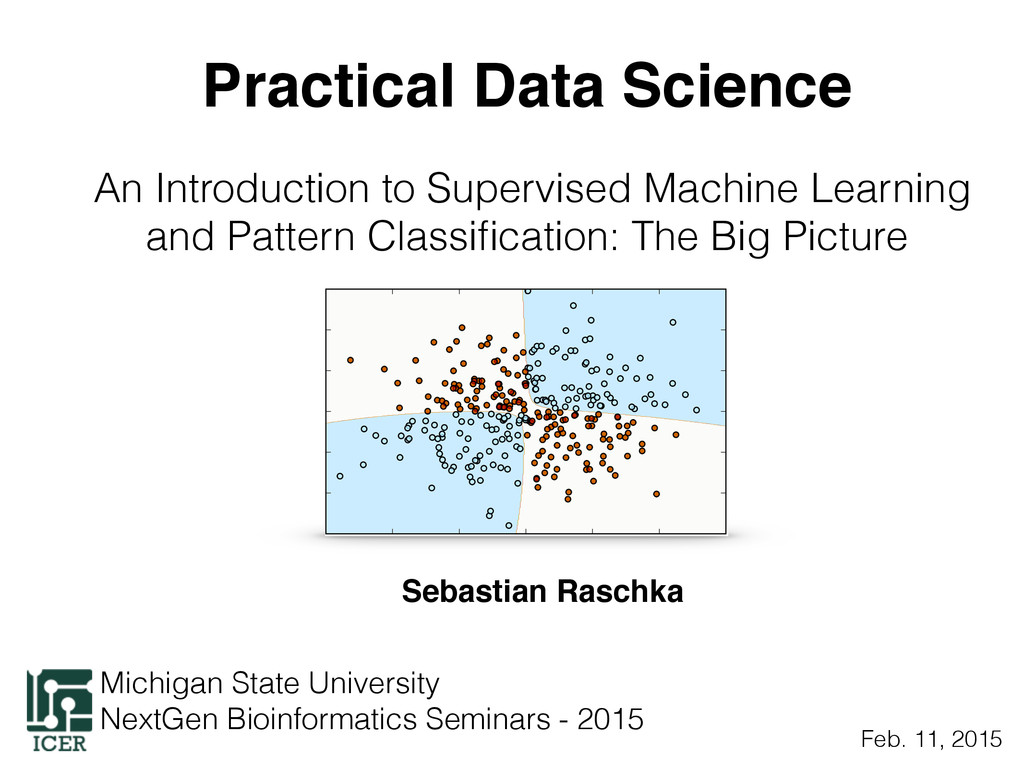
Practical Data Science. An Introduction to Supervised Machine Learning and Pattern Classification: The Big Picture @ NextGen Bioinformatics Michigan State
Practical Data Science. Slides of an 1 hour introductory talk about predictive modeling using Machine Learning with a focus on supervised learning.
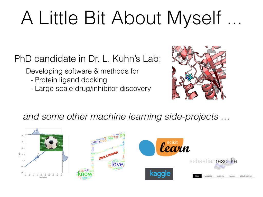
for - Protein ligand docking - Large scale drug/inhibitor discovery PhD candidate in Dr. L. Kuhn’s Lab: and some other machine learning side-projects …
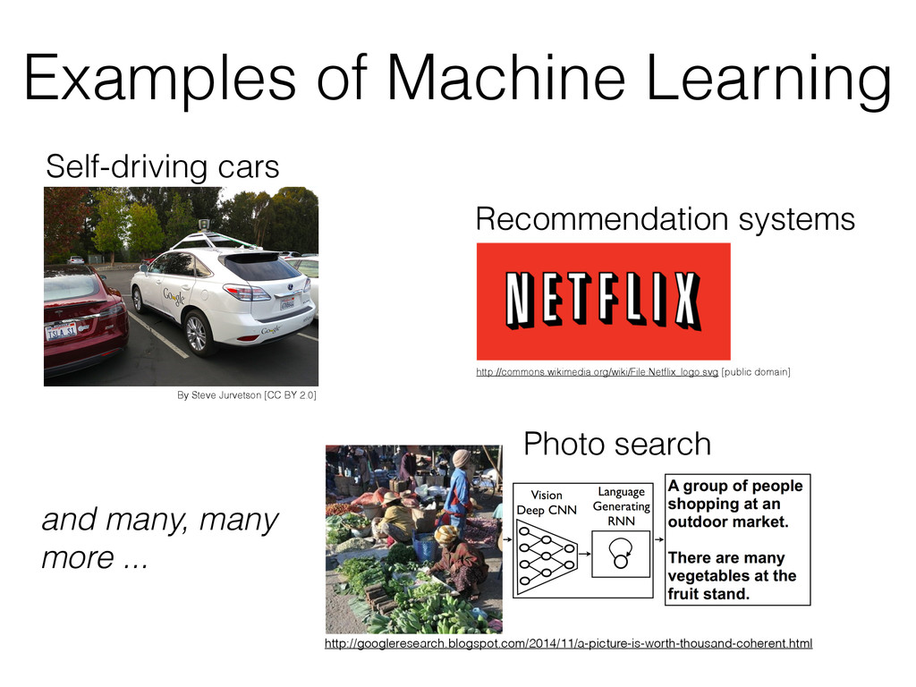
2.0] Self-driving cars Photo search and many, many more ... Recommendation systems http://commons.wikimedia.org/wiki/File:Netflix_logo.svg [public domain]
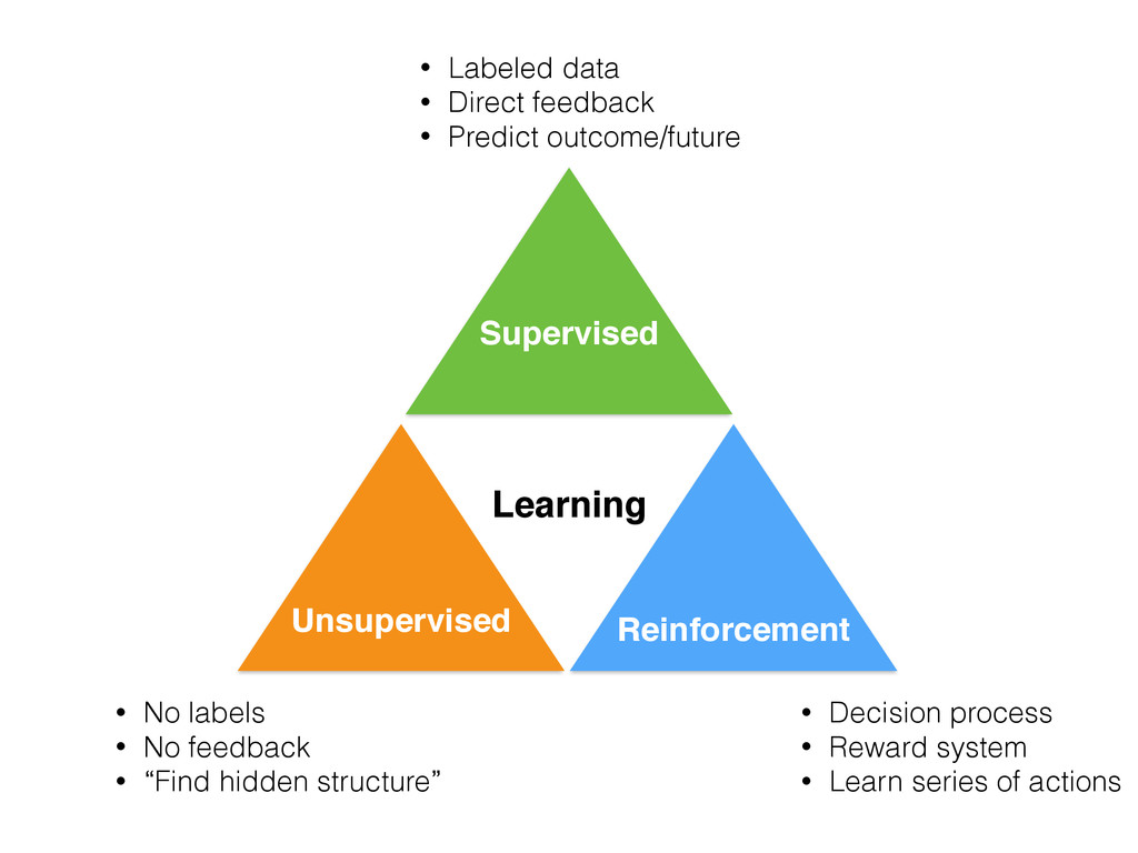
Classification: [SVM on 2 classes of the Wine dataset] Regression: [Soccer Fantasy Score prediction] Today’s topic Supervised Learning Unsupervised Learning
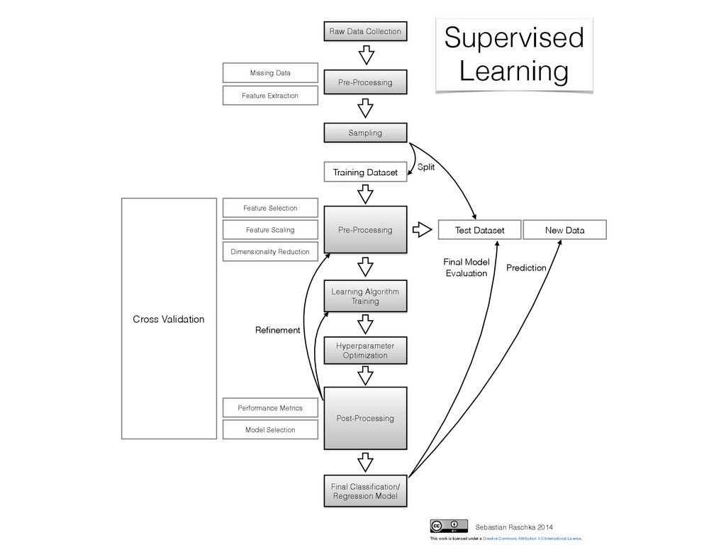
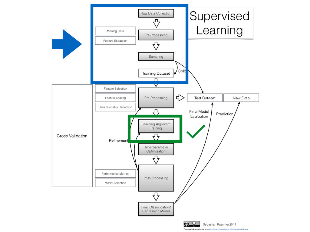
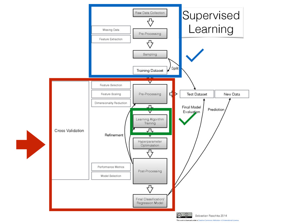
Collection Pre-Processing Sampling Test Dataset Training Dataset Learning Algorithm Training Post-Processing Cross Validation Final Classification/ Regression Model New Data Pre-Processing Refinement Prediction Split Supervised Learning Sebastian Raschka 2014 Missing Data Performance Metrics Model Selection Hyperparameter Optimization This work is licensed under a Creative Commons Attribution 4.0 International License. Final Model Evaluation
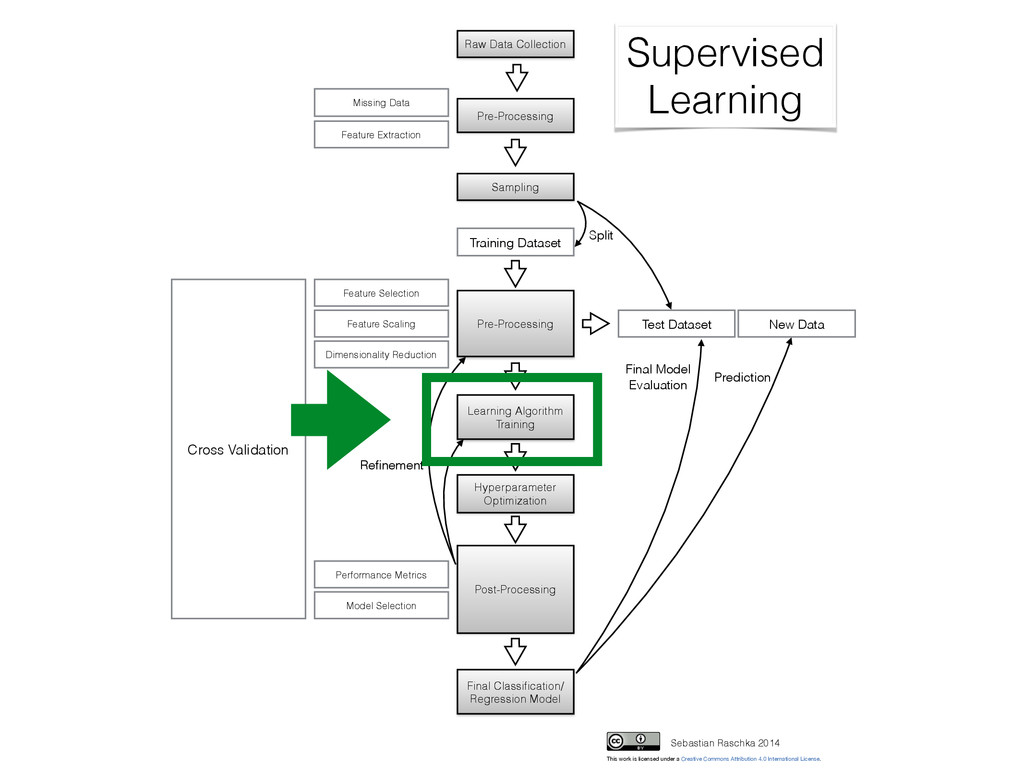
Collection Pre-Processing Sampling Test Dataset Training Dataset Learning Algorithm Training Post-Processing Cross Validation Final Classification/ Regression Model New Data Pre-Processing Refinement Prediction Split Supervised Learning Sebastian Raschka 2014 Missing Data Performance Metrics Model Selection Hyperparameter Optimization This work is licensed under a Creative Commons Attribution 4.0 International License. Final Model Evaluation
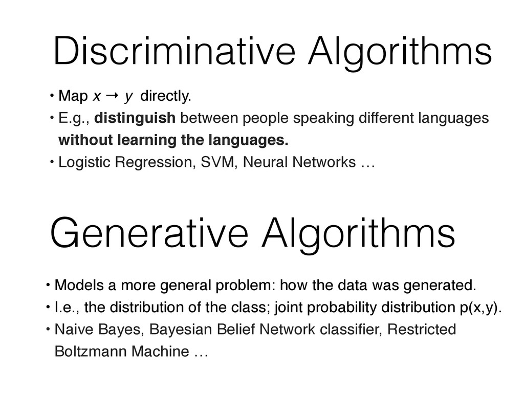
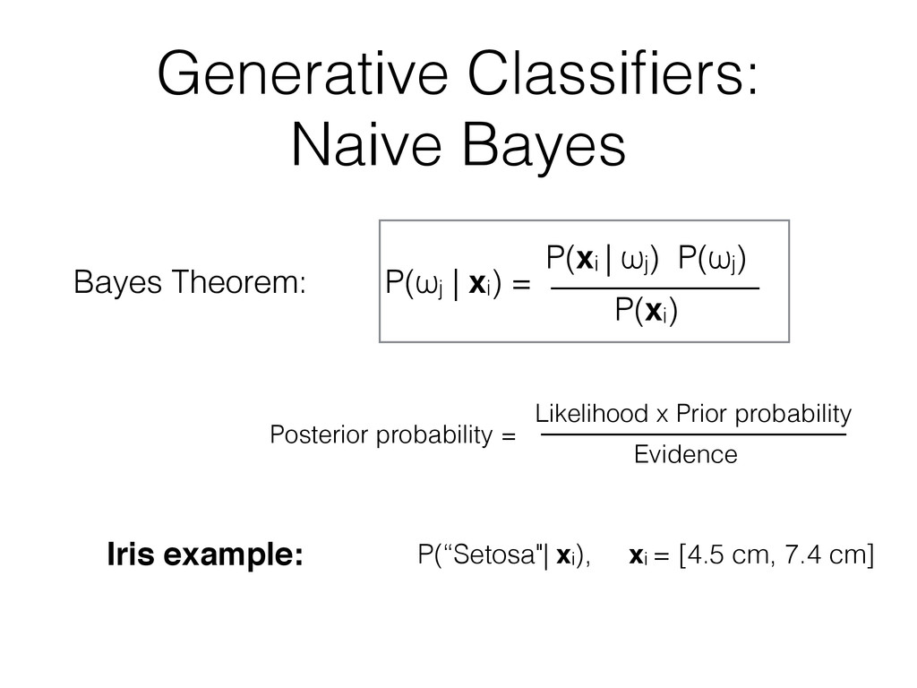
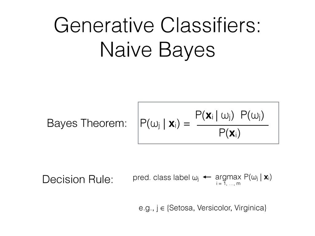
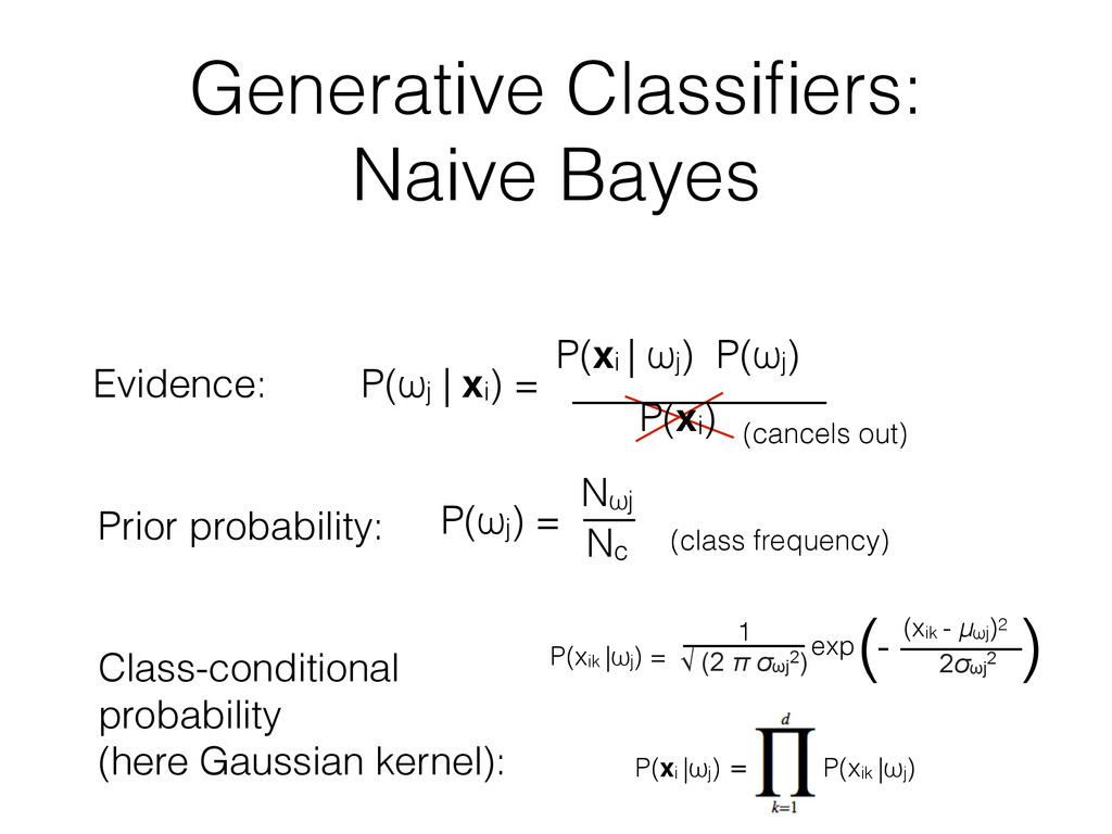
how the data was generated. • I.e., the distribution of the class; joint probability distribution p(x,y). • Naive Bayes, Bayesian Belief Network classifier, Restricted Boltzmann Machine … • Map x → y directly. • E.g., distinguish between people speaking different languages without learning the languages. • Logistic Regression, SVM, Neural Networks …
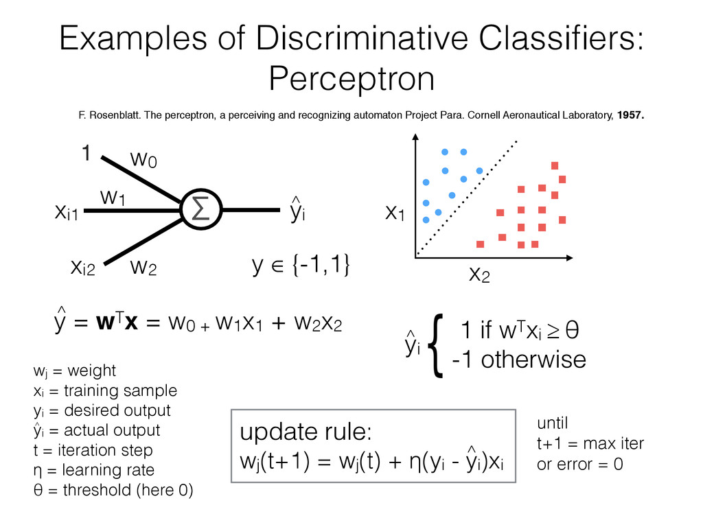
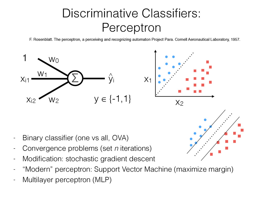
yi y = wTx = w0 + w1x1 + w2x2 1 F. Rosenblatt. The perceptron, a perceiving and recognizing automaton Project Para. Cornell Aeronautical Laboratory, 1957. x1 x2 y ∈ {-1,1} w0 wj = weight xi = training sample yi = desired output yi = actual output t = iteration step η = learning rate θ = threshold (here 0) update rule: wj(t+1) = wj(t) + η(yi - yi)xi 1 if wTxi ≥ θ -1 otherwise ^ ^ ^ ^ yi ^ until t+1 = max iter or error = 0
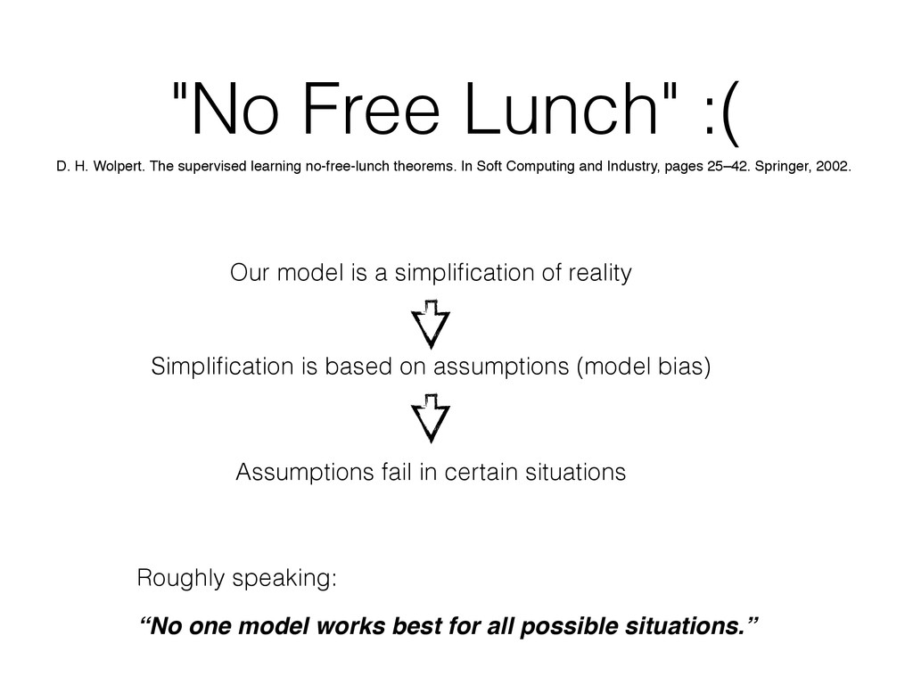
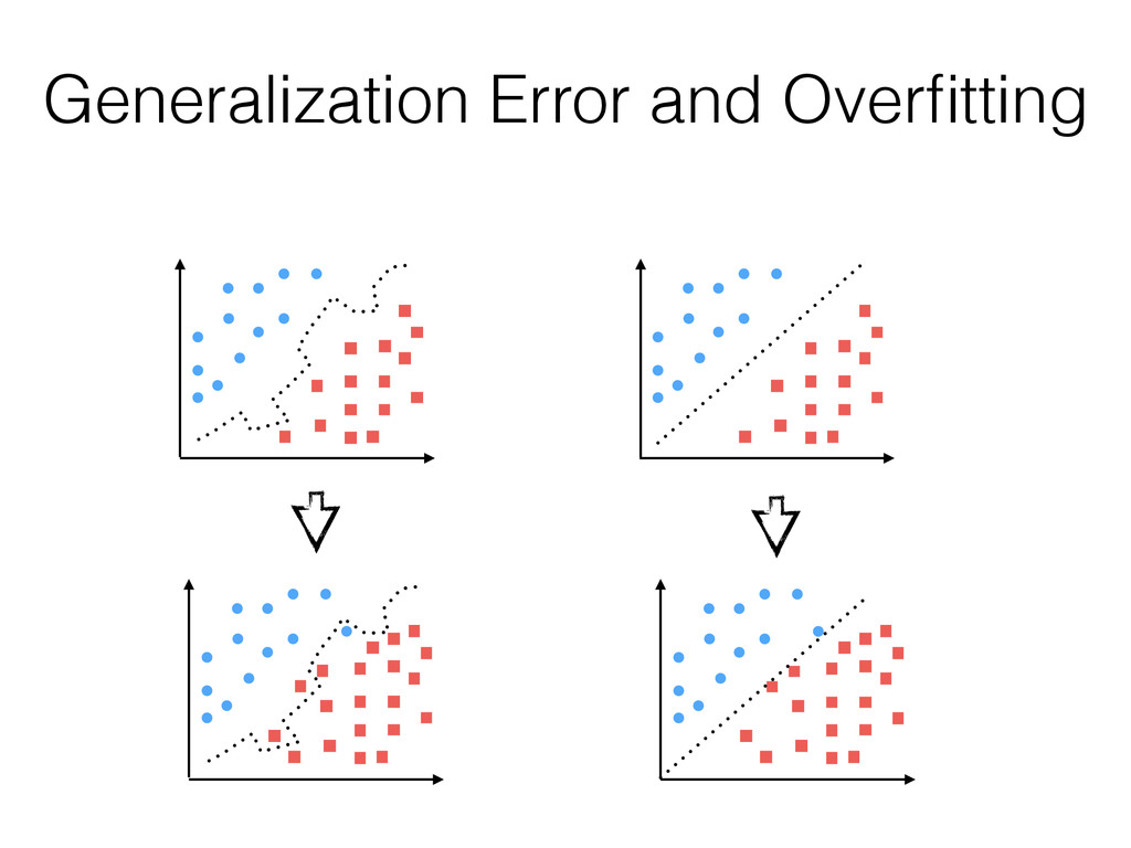
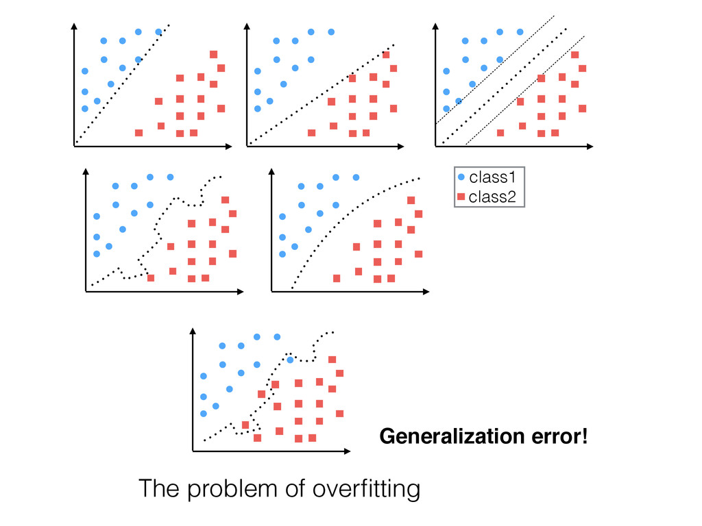
best for all possible situations.” Our model is a simplification of reality Simplification is based on assumptions (model bias) Assumptions fail in certain situations D. H. Wolpert. The supervised learning no-free-lunch theorems. In Soft Computing and Industry, pages 25–42. Springer, 2002.
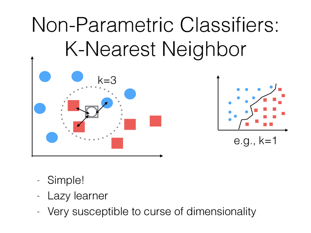
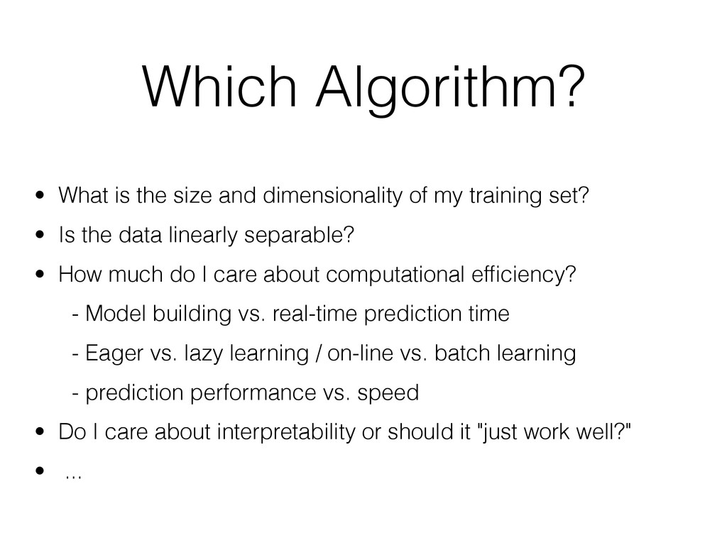
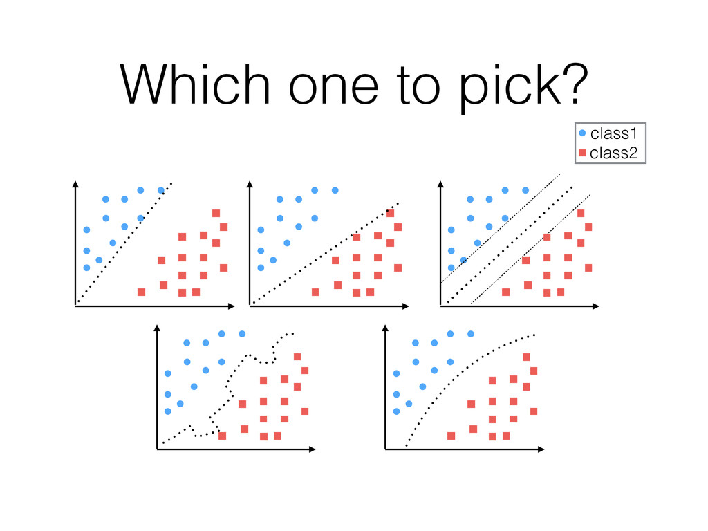
my training set? • Is the data linearly separable? • How much do I care about computational efficiency? - Model building vs. real-time prediction time - Eager vs. lazy learning / on-line vs. batch learning - prediction performance vs. speed • Do I care about interpretability or should it "just work well?" • ...
Collection Pre-Processing Sampling Test Dataset Training Dataset Learning Algorithm Training Post-Processing Cross Validation Final Classification/ Regression Model New Data Pre-Processing Refinement Prediction Split Supervised Learning Sebastian Raschka 2014 Missing Data Performance Metrics Model Selection Hyperparameter Optimization This work is licensed under a Creative Commons Attribution 4.0 International License. Final Model Evaluation
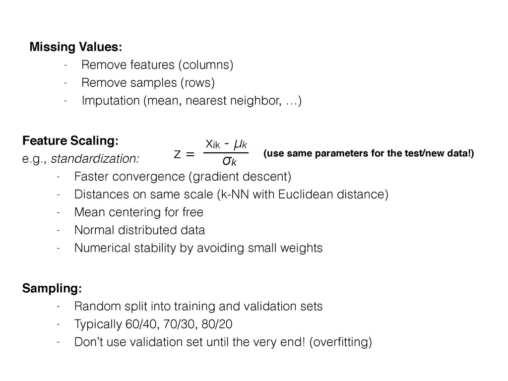
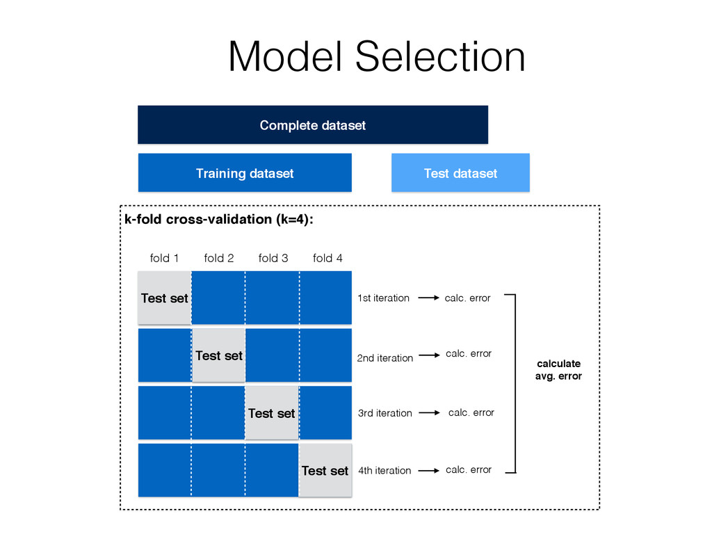
- Imputation (mean, nearest neighbor, …) Sampling: - Random split into training and validation sets - Typically 60/40, 70/30, 80/20 - Don’t use validation set until the very end! (overfitting) Feature Scaling: e.g., standardization: - Faster convergence (gradient descent) - Distances on same scale (k-NN with Euclidean distance) - Mean centering for free - Normal distributed data - Numerical stability by avoiding small weights z = xik - μk σk (use same parameters for the test/new data!)
Collection Pre-Processing Sampling Test Dataset Training Dataset Learning Algorithm Training Post-Processing Cross Validation Final Classification/ Regression Model New Data Pre-Processing Refinement Prediction Split Supervised Learning Sebastian Raschka 2014 Missing Data Performance Metrics Model Selection Hyperparameter Optimization This work is licensed under a Creative Commons Attribution 4.0 International License. Final Model Evaluation
Collection Pre-Processing Sampling Test Dataset Training Dataset Learning Algorithm Training Post-Processing Cross Validation Final Classification/ Regression Model New Data Pre-Processing Refinement Prediction Split Supervised Learning Sebastian Raschka 2014 Missing Data Performance Metrics Model Selection Hyperparameter Optimization This work is licensed under a Creative Commons Attribution 4.0 International License. Final Model Evaluation
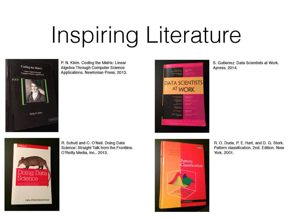
Through Computer Science Applications. Newtonian Press, 2013. R. Schutt and C. O’Neil. Doing Data Science: Straight Talk from the Frontline. O’Reilly Media, Inc., 2013. S. Gutierrez. Data Scientists at Work. Apress, 2014. R. O. Duda, P. E. Hart, and D. G. Stork. Pattern classification. 2nd. Edition. New York, 2001.
![http://commons.wikimedia.org/wiki/ File:American_book_company_1916._letter_envelope-2.JPG#filelinks [public domain] https://flic.kr/p/5BLW6G [CC BY 2.0] Text Recognition](https://files.speakerdeck.com/presentations/560ff726870b42bdb9c7827b62556eb8/slide_3.jpg)
![Unsupervised learning Supervised learning Clustering: [DBSCAN on a toy dataset]](https://files.speakerdeck.com/presentations/560ff726870b42bdb9c7827b62556eb8/slide_8.jpg)
![Error Metrics: Confusion Matrix TP [Linear SVM on sepal/petal lengths]](https://files.speakerdeck.com/presentations/560ff726870b42bdb9c7827b62556eb8/slide_32.jpg)
![Error Metrics TP [Linear SVM on sepal/petal lengths] TN FN](https://files.speakerdeck.com/presentations/560ff726870b42bdb9c7827b62556eb8/slide_33.jpg)
![Questions? [email protected] https://github.com/rasbt @rasbt Thanks!](https://files.speakerdeck.com/presentations/560ff726870b42bdb9c7827b62556eb8/slide_48.jpg)