Estimating Risk: RR, OR, Adjusted OR

A short review of the measures of risk in epidemiological studies.

Transcript

1. 1 Estimating Risk: RR, OR, Adjusted OR Presented by: Pranab Chatterjee Moderated by: Khan Amir Maroof
2. This presentation was made for the Academic Program for Residents at the Department of Community Medicine, University College of Medical Sciences. It is being distributed under a CC – BY – NC (Attribution-Non-Commercial 3.0 Unported) License 2 Estimating Risk: RR, OR, Adjusted OR by Pranab Chatterjee is licensed under a Creative Commons Attribution-NonCommercial 3.0 Unported License.
3. Relative Risk 3
4. Ratio vs Proportions •  Ratio: – Sex ratio: 914 females per 1000 males •  Proportion: – 52% of the population are males 4
5. What is “RISK”? 5 http://xkcd.com/795/
6. RISK? The risk of an event happening is simply the number of those who experience the event divided by the total number of people who are at risk of having that event. 6
7. Absolute Risk •  If rubella infection occurs in a mother 0 – 12 weeks after conception, there is a 51% chance the infant will be affected. 7 http://phil.cdc.gov/phil_images/20030724/28/PHIL_4284_lores.jpg
8. Why absolute risk alone is not sufficient? •  No non-exposed group – no comparator •  Not possible to talk of association 8 http://ddxcomics.com/2011/06/absolute-vs-relative/
9. How do we determine whether a certain disease is associated with a certain exposure? 9 Case Control Studies Cohort Studies
10. Hypothetical Scenario… •  Group A: – Risk of developing disease: 5% •  Group B: – Risk of developing disease: 10% •  How to describe the excess risk in Group B (compared to Group A)? 10
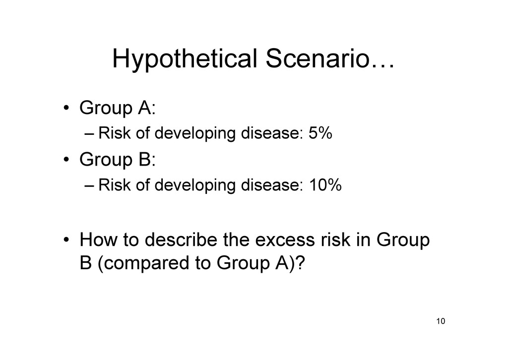
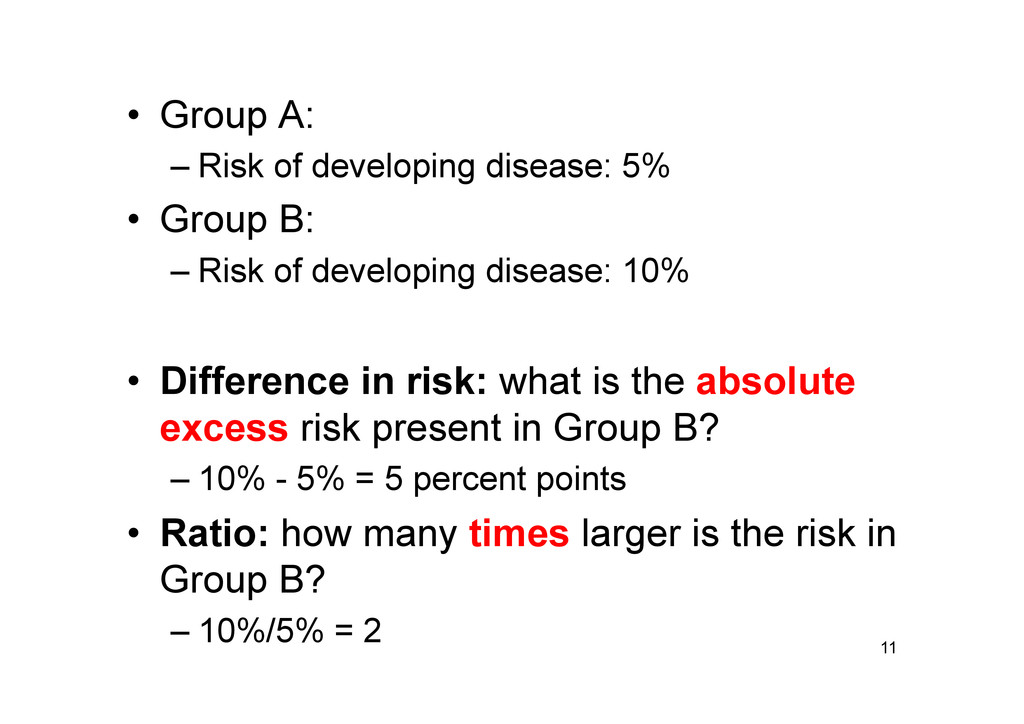
11. •  Group A: – Risk of developing disease: 5% •  Group B: – Risk of developing disease: 10% •  Difference in risk: what is the absolute excess risk present in Group B? – 10% - 5% = 5 percent points •  Ratio: how many times larger is the risk in Group B? – 10%/5% = 2 11
12. Population A Population B Incidence of CAD in smokers 40% 90% Incidence of CAD in non smokers 10% 60% Absolute Risk difference 30% 30% Risk Ratio 4 1.5 12 Gordis L. Epidemiology. Edition 4, Pg 203, table 11-3
13. 13 Population A Population B Incidence of CAD in smokers 40% 60% Incidence of CAD in non smokers 20% 30% Risk Ratio 2 2 Absolute Risk difference 20% 30%
14. Relative Risk (Risk Ratio) •  Ratio of incidence of disease in exposed to the incidence of disease in non exposed. 14
15. Then follow-up to see whether Disease + Disease - Incidence First identify Exposure + a b a/(a+b) Exposure - c d c/(c+d) Relative risk = Incidence in exposed Incidence in non-exposed RR = a/(a+b) c/(c+d) 15
16. Points to Ponder •  Interpreting the RR: – RR = 1 – RR < 1 – RR > 1 •  Incidence is essential: – COHORT STUDIES ONLY 16
17. Odds Ratio 17
18. Chances vs Odds •  You have: 10 marbles in a bag – 2 blue marbles – 3 red marbles – 5 green marbles •  What are your chances (probability) of picking a blue marble? 18
19. Odds •  Ratio of the probability that an event WILL occur to the probability that it will NOT. 19
20. Chances vs Odds •  You have: 10 marbles in a bag – 2 blue marbles – 3 red marbles – 5 green marbles •  What are your odds of picking a blue marble? 20
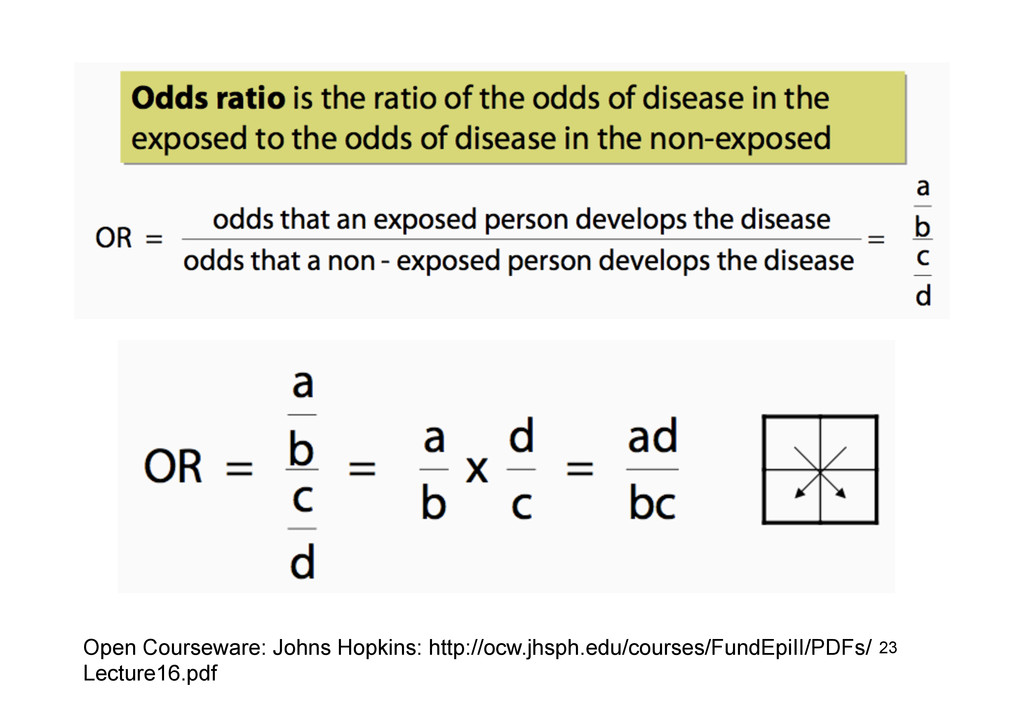
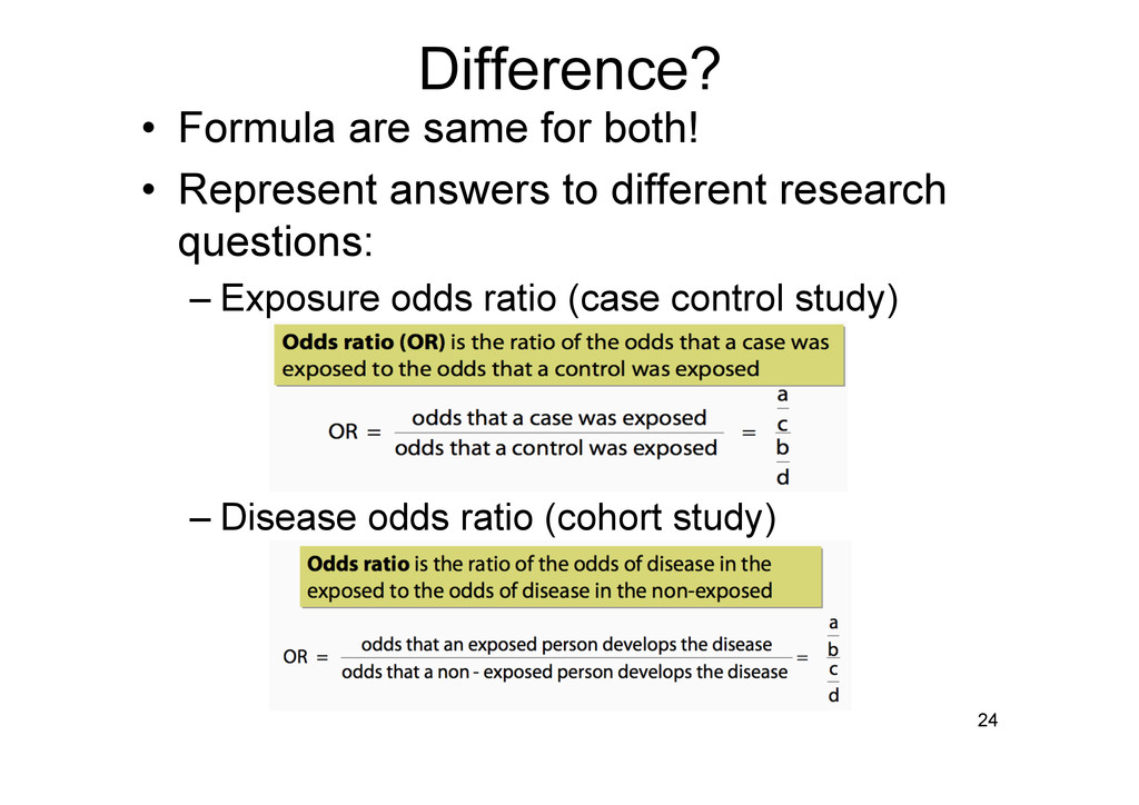
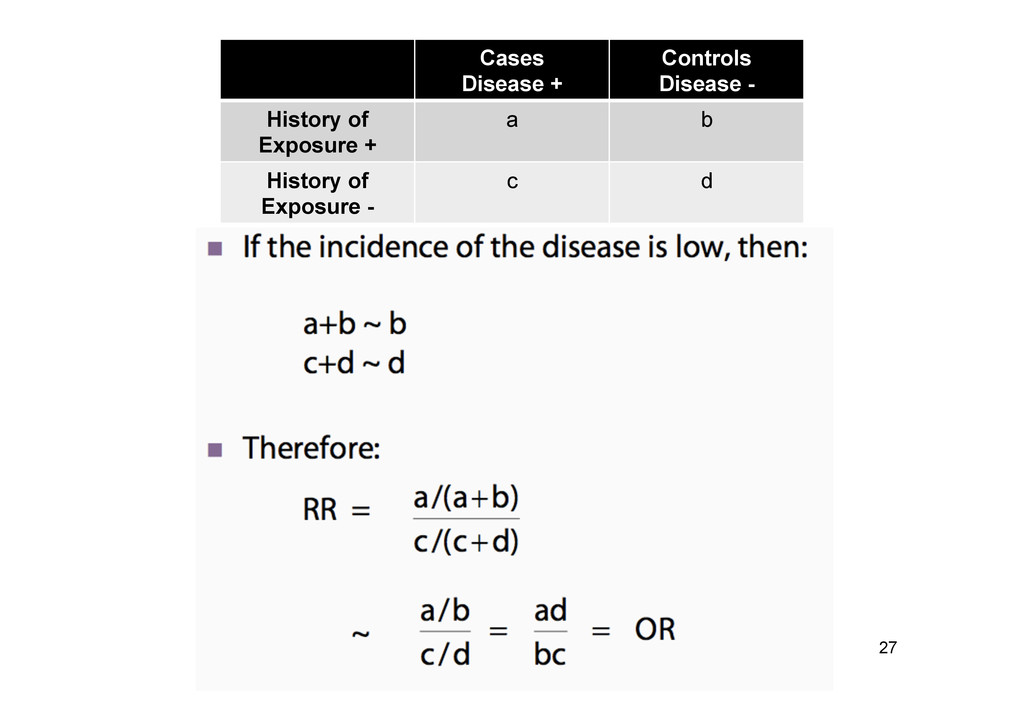
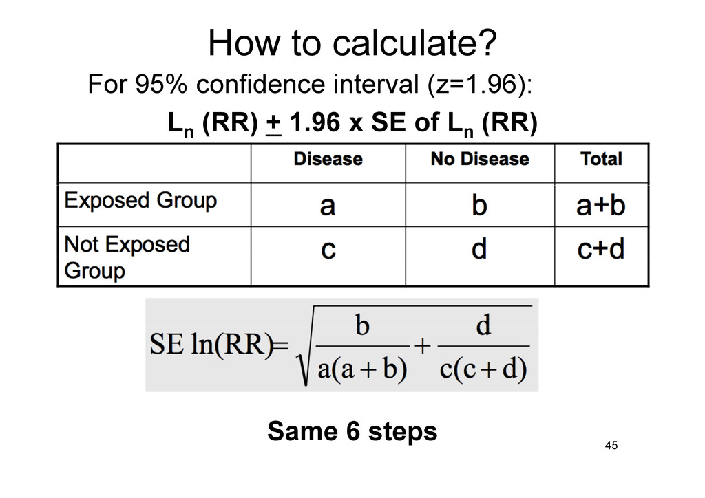
21. OR in Case Control Studies 21 Cases Disease + Controls Disease - History of Exposure + a b History of Exposure - c d Open Courseware: Johns Hopkins: http://ocw.jhsph.edu/courses/FundEpiII/PDFs/ Lecture16.pdf
22. OR in Cohort Studies •  Odds that an exposed person develops the disease? – a/b •  Odds that a non-exposed person develops the disease? – c/d 22 Disease + Disease - Exposure + a b Exposure - c d
23. 23 Open Courseware: Johns Hopkins: http://ocw.jhsph.edu/courses/FundEpiII/PDFs/ Lecture16.pdf
24. Difference? •  Formula are same for both! •  Represent answers to different research questions: – Exposure odds ratio (case control study) – Disease odds ratio (cohort study) 24
25. The Philosophical Premise 25 = (Lung CA + Smoking +) x (Lung CA – Smoking -) (Lung CA+ Smoking -) x (Lung CA – Smoking +) Cases (Lung CA) Disease + Controls (Lung CA) Disease - Exposure (Smoking) + a b Exposure (Smoking) - c d
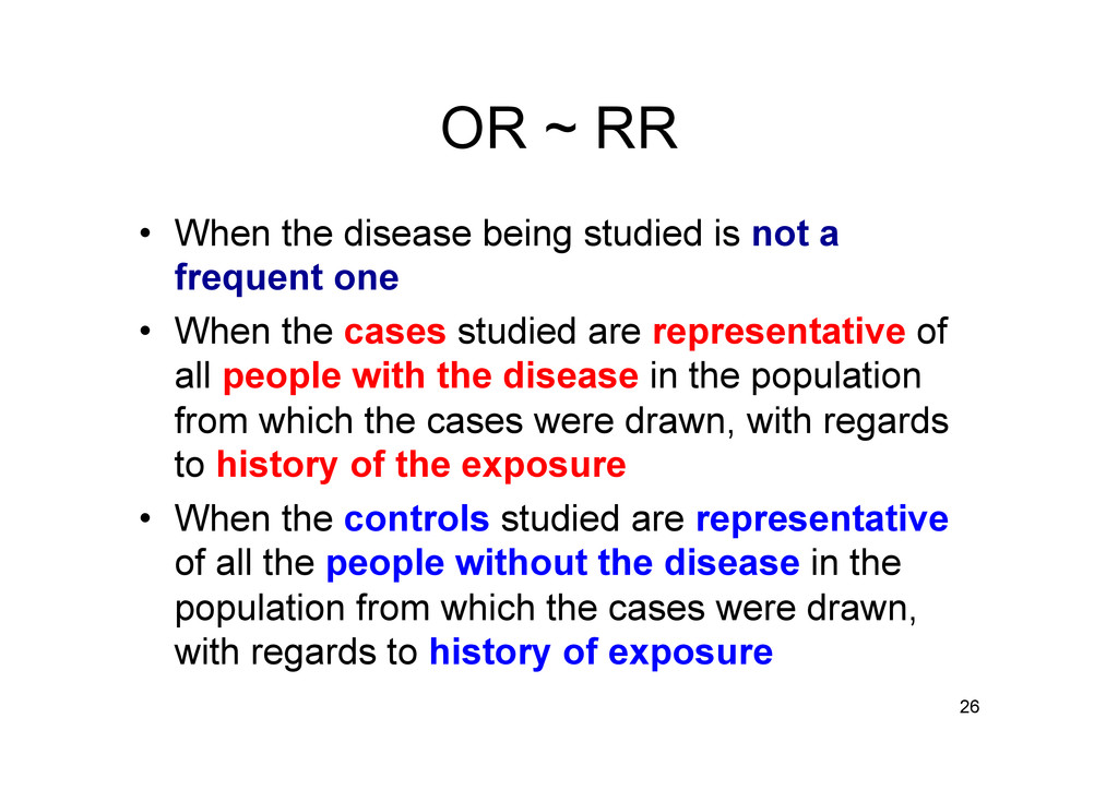
26. OR ~ RR •  When the disease being studied is not a frequent one •  When the cases studied are representative of all people with the disease in the population from which the cases were drawn, with regards to history of the exposure •  When the controls studied are representative of all the people without the disease in the population from which the cases were drawn, with regards to history of exposure 26
27. 27 Cases Disease + Controls Disease - History of Exposure + a b History of Exposure - c d
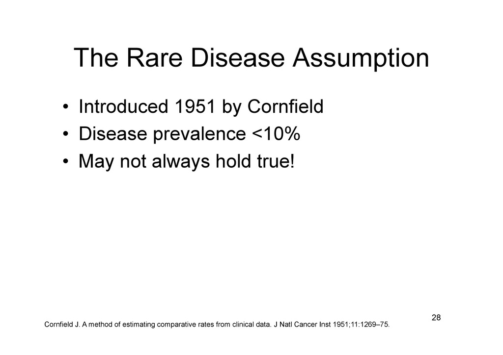
28. The Rare Disease Assumption •  Introduced 1951 by Cornfield •  Disease prevalence <10% •  May not always hold true! 28 Cornfield J. A method of estimating comparative rates from clinical data. J Natl Cancer Inst 1951;11:1269–75.
29. An example: Common Disease •  OR = (69*143)/(22*209) = 2.15 •  RR = (143/352)/(22/91) = 1.68 29 Neck pain No Neck Pain Own a cell phone 143 209 Don’t own a cell phone 22 69
30. An Example: Rare Disease •  OR = (5*88)/(3*347) = 0.42267 •  RR = (5/352)/(3/91) = 0.43087 30
31. Confidence Intervals 31
32. The Philosophy of CI – How to deal with the uncertainty inherent in results derived from data that is in itself a randomly selected subset of a population? – 100 samples from same population: 95 times their CI contains the true mean value! 32
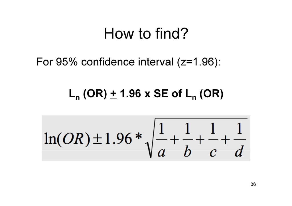
33. Confidence Interval of OR •  The usual form: Point estimate + Confidence coefficient x standard error •  However, for odds ratio, CI is calculated on the natural log scale. Then reversed on the exponential scale… WHY? 33
34. OR: Right Skew 34 Dispersion of Odds Ratio on multiple sampling from the same universe
35. ln OR: Normal Distribution 35 Dispersion of the natural logarithm of the same Odds Ratio obtained on multiple sampling from the same universe as in the preceding slide
36. How to find? For 95% confidence interval (z=1.96): Ln (OR) + 1.96 x SE of Ln (OR) 36
37. From Data to OR to CI Case control study to determine association of preterm delivery with socioeconomic status. 37
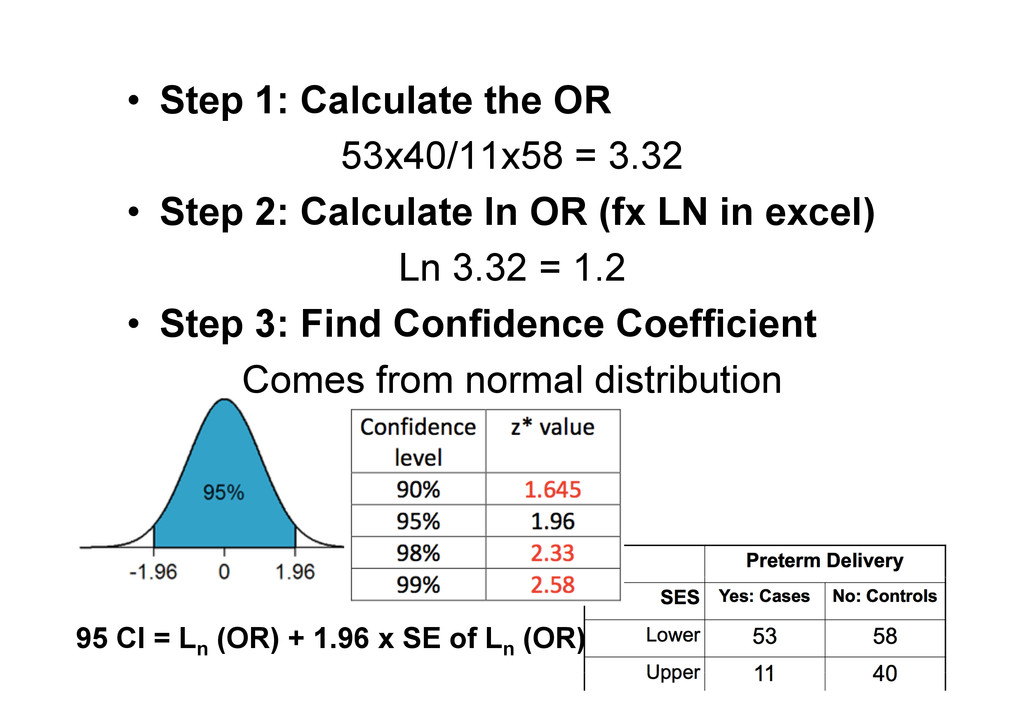
38. •  Step 1: Calculate the OR 53x40/11x58 = 3.32 •  Step 2: Calculate ln OR (fx LN in excel) Ln 3.32 = 1.2 •  Step 3: Find Confidence Coefficient Comes from normal distribution 38 95 CI = Ln (OR) + 1.96 x SE of Ln (OR)
39. •  Step 4: Calculate SE of Ln OR •  Step 5: Find lower & upper limits 39 95 CI = Ln (OR) + 1.96 x SE of Ln (OR)
40. Does it add up? •  OR = 3.32 •  Upper limit of CI = 1.97 •  Lower limit of CI = 0.44 •  So what went wrong? 40
41. THIS ISN’T OVER YET! 41
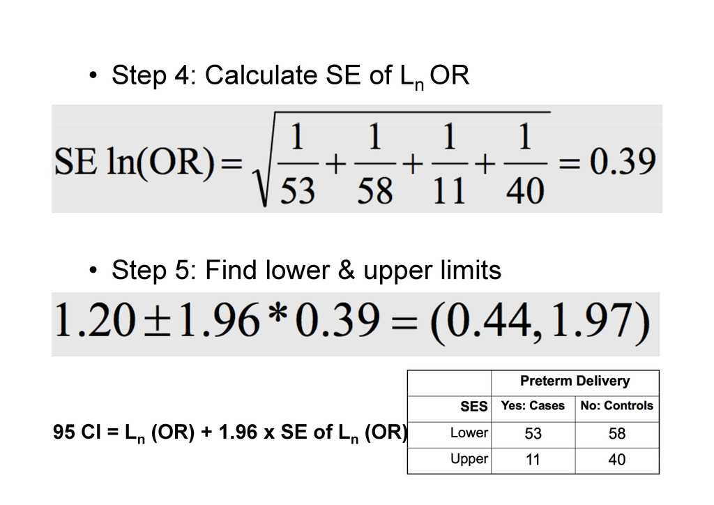
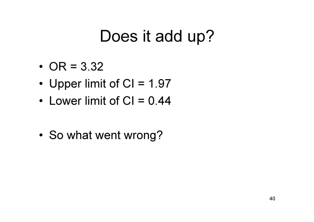
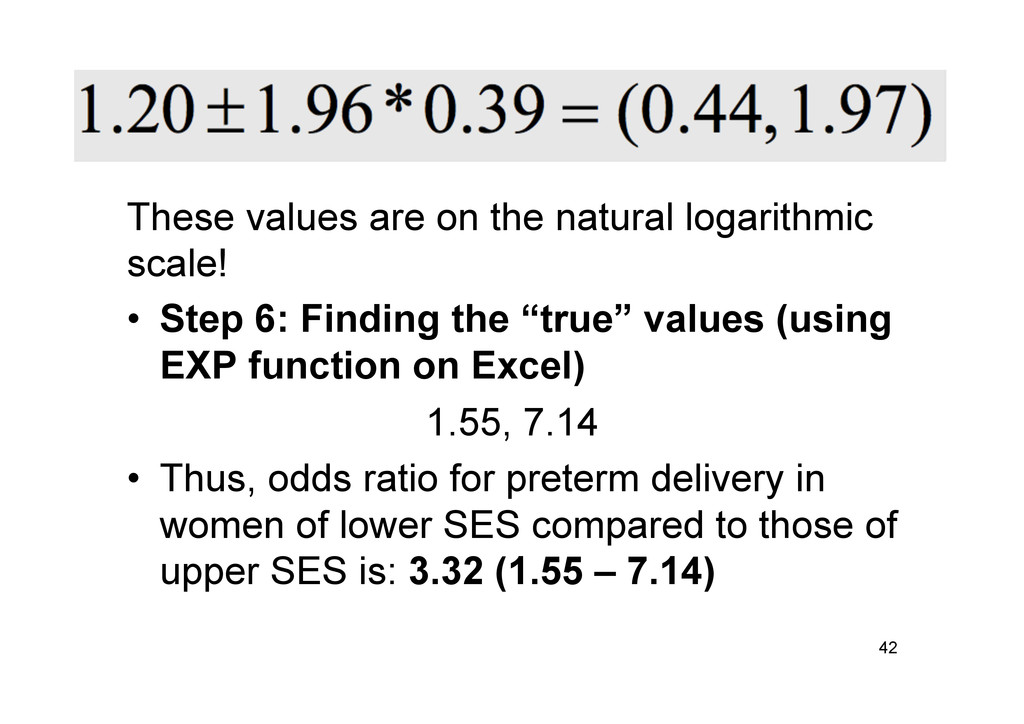
42. These values are on the natural logarithmic scale! •  Step 6: Finding the “true” values (using EXP function on Excel) 1.55, 7.14 •  Thus, odds ratio for preterm delivery in women of lower SES compared to those of upper SES is: 3.32 (1.55 – 7.14) 42
43. Interpreting the OR & Significance •  An OR of 1 = No association •  What does it mean when the CI “breaches” the value of 1? – 3.32 (0.80 – 7.14) [previous example] 43
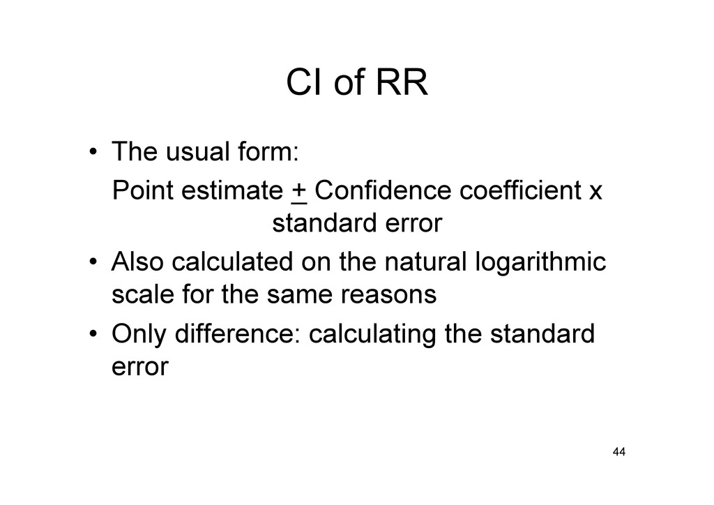
44. CI of RR •  The usual form: Point estimate + Confidence coefficient x standard error •  Also calculated on the natural logarithmic scale for the same reasons •  Only difference: calculating the standard error 44
45. How to calculate? For 95% confidence interval (z=1.96): Ln (RR) + 1.96 x SE of Ln (RR) Same 6 steps 45
46. OR in Matched Case Control Studies 46
47. Matching Changes 2x2 •  When one control is matched to one case, the case and the control forms a pair and are dealt with as such in the contingency tables. •  Concordant Pairs •  Discordant Pairs 47
48. 48 Gordis L. Epidemiology. Edition 4
49. Attributable Risk 49
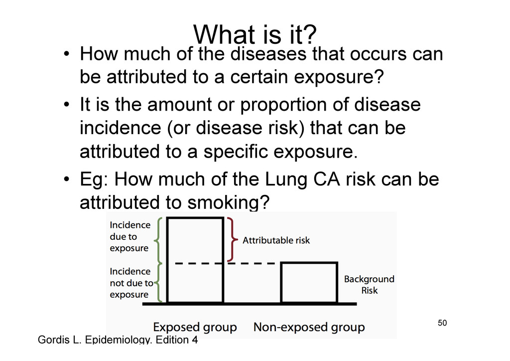
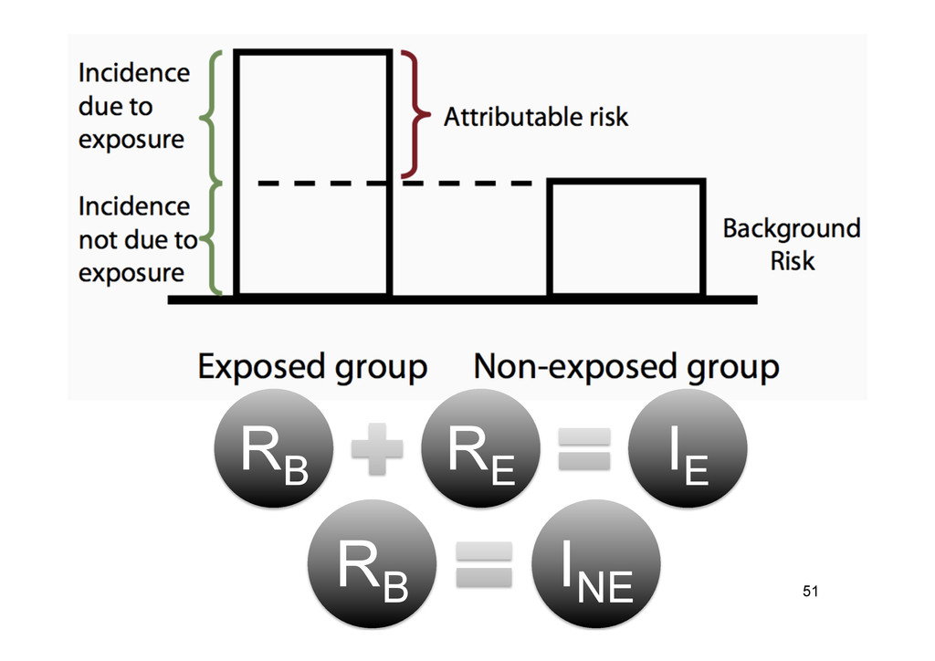
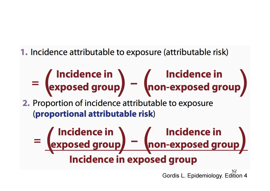
50. What is it? •  How much of the diseases that occurs can be attributed to a certain exposure? •  It is the amount or proportion of disease incidence (or disease risk) that can be attributed to a specific exposure. •  Eg: How much of the Lung CA risk can be attributed to smoking? 50 Gordis L. Epidemiology. Edition 4
51. 51 RB RE IE RB INE
52. 52 Gordis L. Epidemiology. Edition 4
53. Population Attributable Risk •  Populations = Exposed + Unexposed 53 Everyone smokes: PAR = AR Nobody smokes: PAR = 0
54. 54 Gordis L. Epidemiology. Edition 4
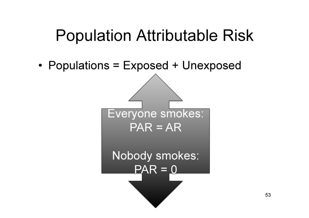
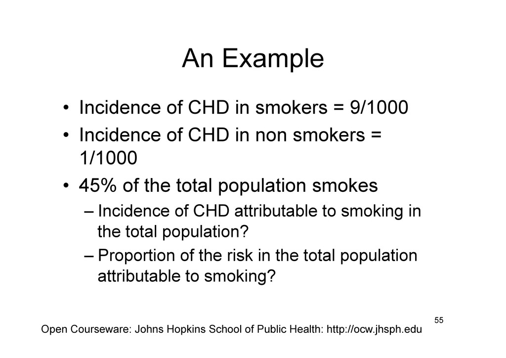
55. An Example •  Incidence of CHD in smokers = 9/1000 •  Incidence of CHD in non smokers = 1/1000 •  45% of the total population smokes – Incidence of CHD attributable to smoking in the total population? – Proportion of the risk in the total population attributable to smoking? 55 Open Courseware: Johns Hopkins School of Public Health: http://ocw.jhsph.edu
56. Step 1: Calculate Incidence of CHD in total population Incidence in smokers x % smokers + Incidence in non-smokers x % non smokers =9/1000 x 0.45 + 1/100 x 0.55 = 4.6 per 1000 56
57. Population Attributable Risk Step 2: Calculate incidence attributable to smoking Incidence in total population – Incidence in non smokers = 4.6 per 1000 – 1 per 1000 = 3.6 per 1000 57
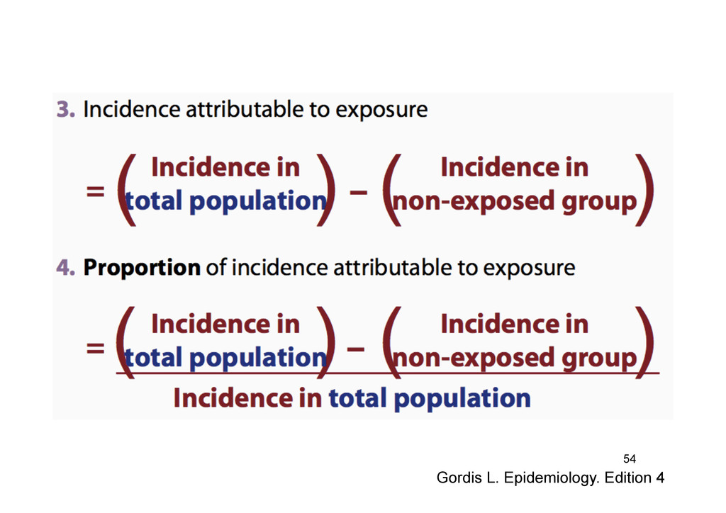
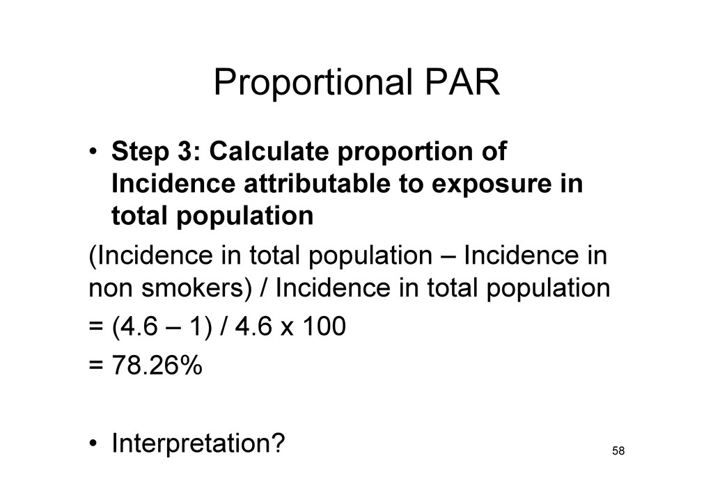
58. Proportional PAR •  Step 3: Calculate proportion of Incidence attributable to exposure in total population (Incidence in total population – Incidence in non smokers) / Incidence in total population = (4.6 – 1) / 4.6 x 100 = 78.26% •  Interpretation? 58
59. Seeing the BIG picture 59 Source: Doll and Peto (1976). BMJ, 2:1525. Philosophical Premise and Public Health Significance
60. Reviewing Confounding 60
61. An Example Dental Caries <15 yrs SDHP F in H2 O 61 1990: 10% 2010: 5% Adapted from: Rothman KJ, Greenland S, Lash TL. Modern Epidemiology. Edition 3
62. 62 Ooh! A time machine!
63. An Example Dental Caries <15 yrs SDHP 63 1990: 10% 2010: 7% 2010: 5%
64. Effect vs Association A: 5% B: 8% Cx X Ca Cx Fwater Ca 64 Starting 10% Starting 10%
65. Association and Causation 65 http://xkcd.com/552/
66. Interaction 66
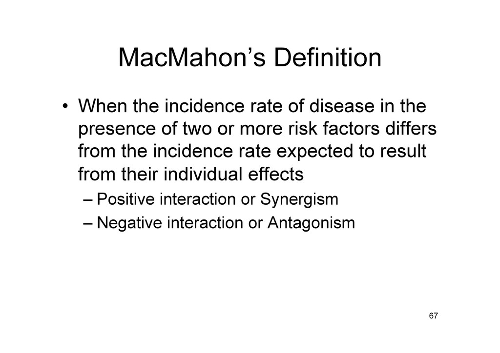
67. MacMahon’s Definition •  When the incidence rate of disease in the presence of two or more risk factors differs from the incidence rate expected to result from their individual effects – Positive interaction or Synergism – Negative interaction or Antagonism 67
68. Incidence Rates and Exposure Pattern Factor A - Factor A + Factor B - 3.0 9.0 Factor B + 15.0 ? 68
69. Additive Model 69 Factor A - Factor A + Factor B - 3.0 9.0 Factor B + 15.0 21.0 Factor A - Factor A + Factor B - 0 6.0 Factor B + 12.0 18.0 Attributable Risk
70. Multiplicative Model 70 Factor A - Factor A + Factor B - 3.0 9.0 Factor B + 15.0 45.0 Factor A - Factor A + Factor B - 1 3.0 Factor B + 5.0 15.0 Relative Risk
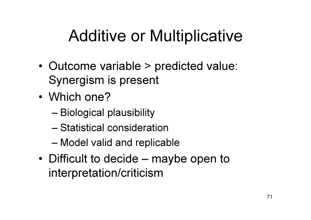
71. Additive or Multiplicative •  Outcome variable > predicted value: Synergism is present •  Which one? – Biological plausibility – Statistical consideration – Model valid and replicable •  Difficult to decide – maybe open to interpretation/criticism 71
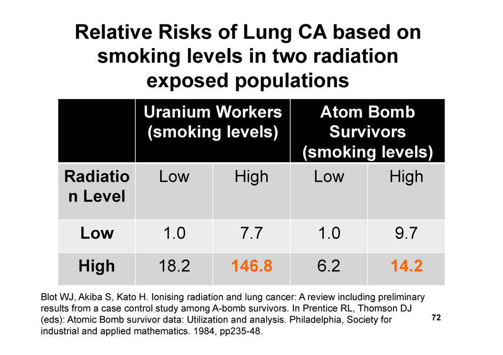
72. Uranium Workers (smoking levels) Atom Bomb Survivors (smoking levels) Radiatio n Level Low High Low High Low 1.0 7.7 1.0 9.7 High 18.2 146.8 6.2 14.2 72 Relative Risks of Lung CA based on smoking levels in two radiation exposed populations Blot WJ, Akiba S, Kato H. Ionising radiation and lung cancer: A review including preliminary results from a case control study among A-bomb survivors. In Prentice RL, Thomson DJ (eds): Atomic Bomb survivor data: Utilization and analysis. Philadelphia, Society for industrial and applied mathematics. 1984, pp235-48.
73. Adjusted Odds Ratio 73
74. Woolf’s Method •  Sampling errors •  Measures of sampling errors: – CI and SE – Coefficient of variance •  Woolf’s method uses coefficient of variance 74 London School of Hygiene and Tropical Medicine: http://conflict.lshtm.ac.uk/page_45.htm
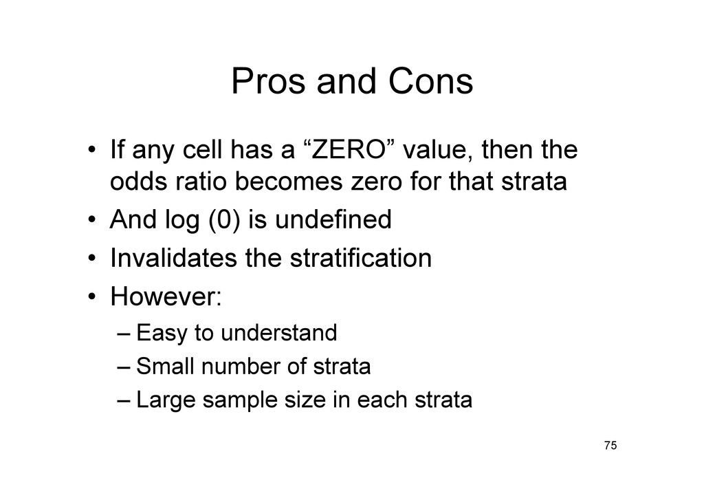
75. Pros and Cons •  If any cell has a “ZERO” value, then the odds ratio becomes zero for that strata •  And log (0) is undefined •  Invalidates the stratification •  However: – Easy to understand – Small number of strata – Large sample size in each strata 75
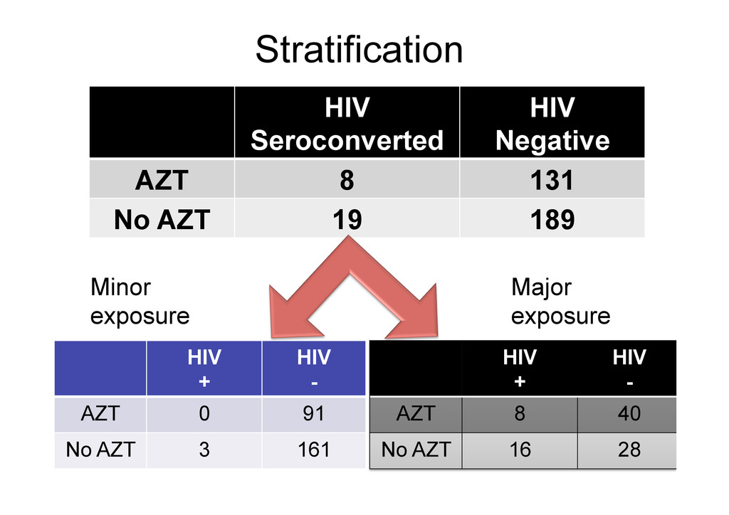
76. Example: PEP for HIV HIV Seroconverted HIV Negative AZT 8 131 No AZT 19 189 76 Li, R. W., & Wong, J. B. (1997). Postexposure treatment of HIV. N Engl J Med, 337(7), 499-500; author reply 501. ORcrude =0.61 95% CI = 0.26 – 1.4
77. Confounders? 77 AZT PEP HIV Seroconversion Severity of exposure
78. Stratification 78 HIV Seroconverted HIV Negative AZT 8 131 No AZT 19 189 HIV + HIV - AZT 0 91 No AZT 3 161 HIV + HIV - AZT 8 40 No AZT 16 28 Minor exposure Major exposure
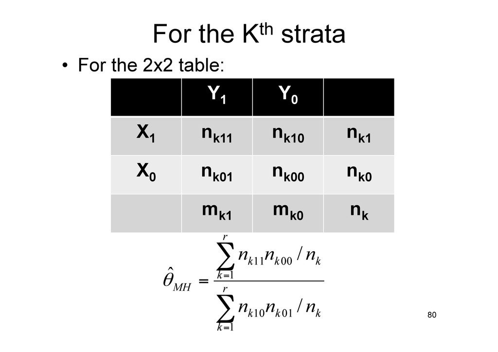
79. The Mantel Haenszel Common Odds Ratio •  Landmark paper in 1959 •  Weighted mean of the odds ratio of the individual strata. (hence “common”) 79 Mantel, N.; Haenszel, W. (1959), "Statistical aspects of the analysis of data from the retrospective analysis of disease", Journal of the National Cancer Institute 22 (4): 719–748, PMID 13655060
80. For the Kth strata •  For the 2x2 table: 80 ∑ ∑ = = = r k k k k r k k k k MH n n n n n n 1 01 10 1 00 11 / / ˆ θ Y1 Y0 X1 nk11 nk10 nk1 X0 nk01 nk00 nk0 mk1 mk0 nk
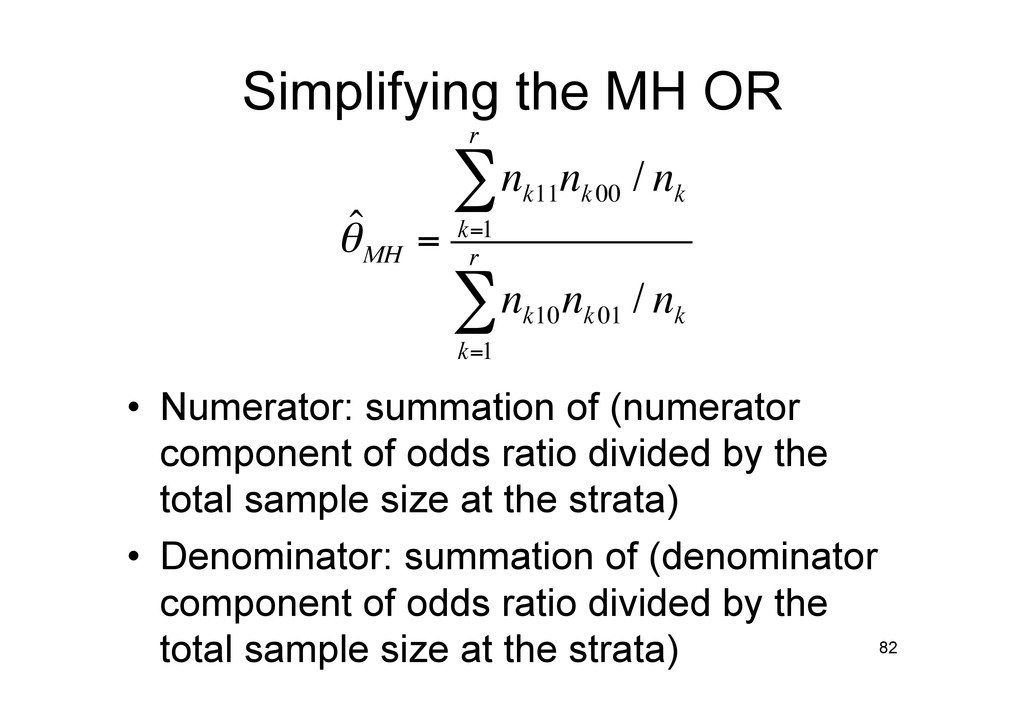
82. Simplifying the MH OR •  Numerator: summation of (numerator component of odds ratio divided by the total sample size at the strata) •  Denominator: summation of (denominator component of odds ratio divided by the total sample size at the strata) 82 ˆ θMH = n k11 n k00 / n k k=1 r ∑ n k10 n k01 / n k k=1 r ∑
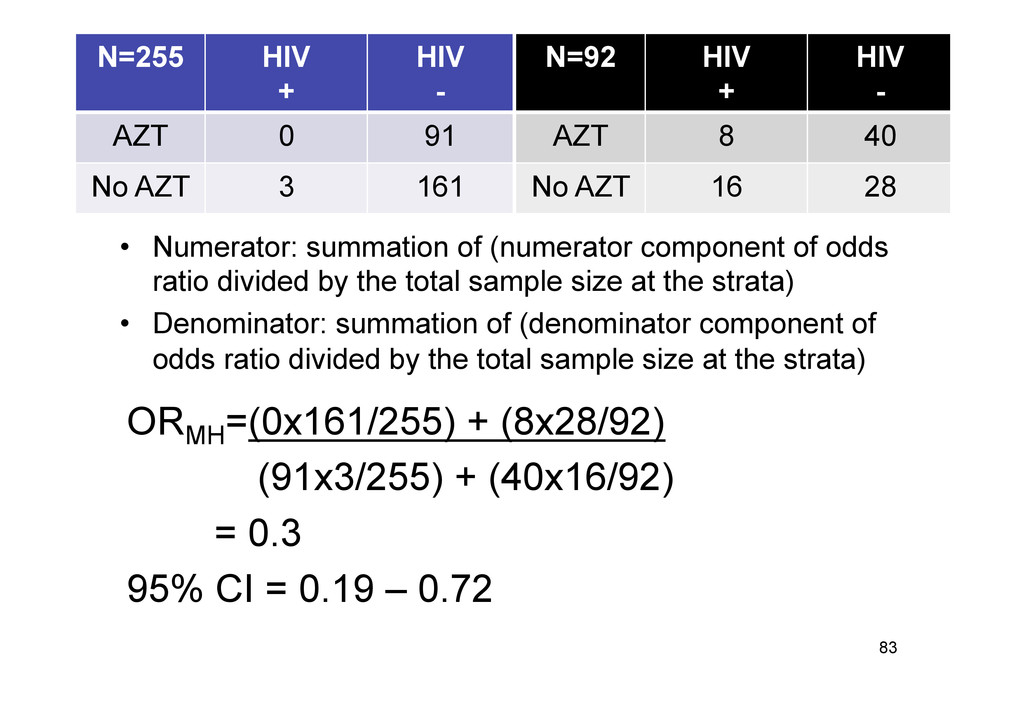
83. ORMH =(0x161/255) + (8x28/92) (91x3/255) + (40x16/92) = 0.3 95% CI = 0.19 – 0.72 83 N=255 HIV + HIV - AZT 0 91 No AZT 3 161 N=92 HIV + HIV - AZT 8 40 No AZT 16 28 •  Numerator: summation of (numerator component of odds ratio divided by the total sample size at the strata) •  Denominator: summation of (denominator component of odds ratio divided by the total sample size at the strata)
84. Pros and Cons •  Difficult to conceptualize •  Can deal with large number of strata •  Can deal with cell values of ZERO •  Easy to compute •  Most commonly used approach to form adjusted summary estimates 84
85. OR & RR in Current Research 85
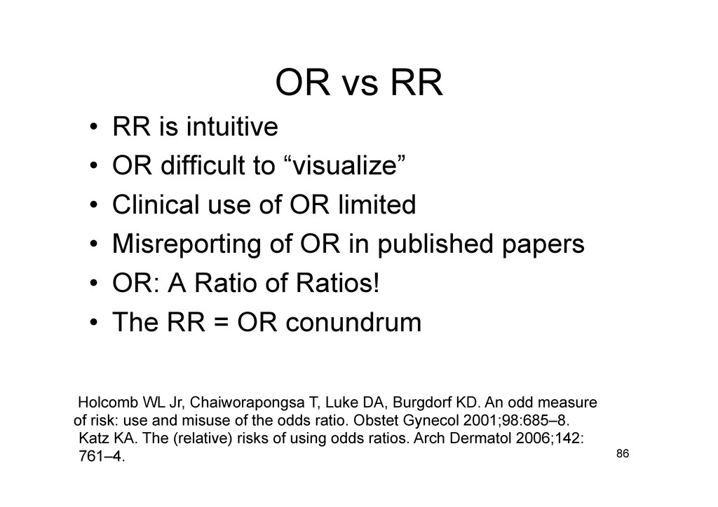
86. OR vs RR •  RR is intuitive •  OR difficult to “visualize” •  Clinical use of OR limited •  Misreporting of OR in published papers •  OR: A Ratio of Ratios! •  The RR = OR conundrum 86 Holcomb WL Jr, Chaiworapongsa T, Luke DA, Burgdorf KD. An odd measure of risk: use and misuse of the odds ratio. Obstet Gynecol 2001;98:685–8. Katz KA. The (relative) risks of using odds ratios. Arch Dermatol 2006;142: 761–4.