An Introduction to Basics of Data Science Part 1

Part 1: basic intro to collaborative filtering, classification, using pandas and sci-kit learn

Transcript

1. Introduction to Data Science First steps into machine learning and its applications !/serhanbaker/datasci-presentation
2. Contents Vocabulary Data Modeling and Data Preparation Recommendation Systems with Collaborative Filtering - Manhattan Distance - Euclidean Distance - Pearson Correlation Coefficient - Cosine Similarity - Sample Cases - K Nearest Neighbor Linear Regression and Sample Code Probability and Bayes Law - Naïve Bayes Classification Using scikit-learn with SVM Sample Code K-Means Clustering Sample Code (@ repository)
3. Terms Statistics is concerned with probabilistic models, specifically inference on these models using data. Artificial Intelligence is anything that is concerned with intelligence in computers. So, it includes lots of things. Data Mining is applied machine learning. It focuses more on the practical aspects of deploying machine learning algorithms on large datasets. Machine Learning is concerned with predicting a particular outcome given some data. It looks like statistics. Focuses on computational efficiency and large datasets.
4. In Short… Statistics quantifies numbers Artificial Intelligence behaves and reasons Data Mining explains patterns Machine Learning predicts with models
5. Machine Learning Topics In general, a machine learning problem has a set of samples of data and then tries to predict properties of unknown data If each sample is more than just one number (multivariate data): Then it’s said that our sample have several attributes (aka features) We can separate learning problems into 2 large categories: • Supervised Learning • Classification • Regression • Unsupervised Learning • Clustering • Density Estimation
6. Supervised Learning Assumes you have a set of data with labels Problem can be either: Classification: Samples belong to two or more classes and we want to learn from already labeled data how to predict the class of unlabeled data. I know what these things are, can I take a known thing, and put it in the right bucket? Handwritten digit recognition example Regression: If the desired output consists of one or more continuous variables, then the task is called regression. Prediction of the length of a salmon as a function of its age and weight.
7. Unsupervised Learning Assumes you have bunch of data with no labels Clustering: I have universe of things. Can I find groups in that universe? Density Estimation: Determine the distribution of data within the input space
8. Entity Disambiguation Are FB, FBOOK, FACEBOOK the same company? Are Tr, TUR, Turkey the same country? Turkey (animal), Turkey (country) which is which? NY? NYC? New York?
9. Data Modeling How the Data Look Like user_id name age gender 101 Luke 26 male 102 Chloe 17 female 103 Leia 23 female book_id title year author genre Xa2Jh1 Great Gatsby 1925 F. Scott Fitzgerald fiction Zb8Km7 A Farewell to Arms 1926 Ernest Hemingway fiction Ao9Cs0 A Beautiful Mind 1994 Sylvia Nasar biography user_id book_id visited rented purchased rating 101 Ao9Cs0 Y N Y 4 103 Xa2Jh1 Y Y N 3 102 Ao9Cs0 Y N N 0 101 Zb8Km7 Y Y Y 5
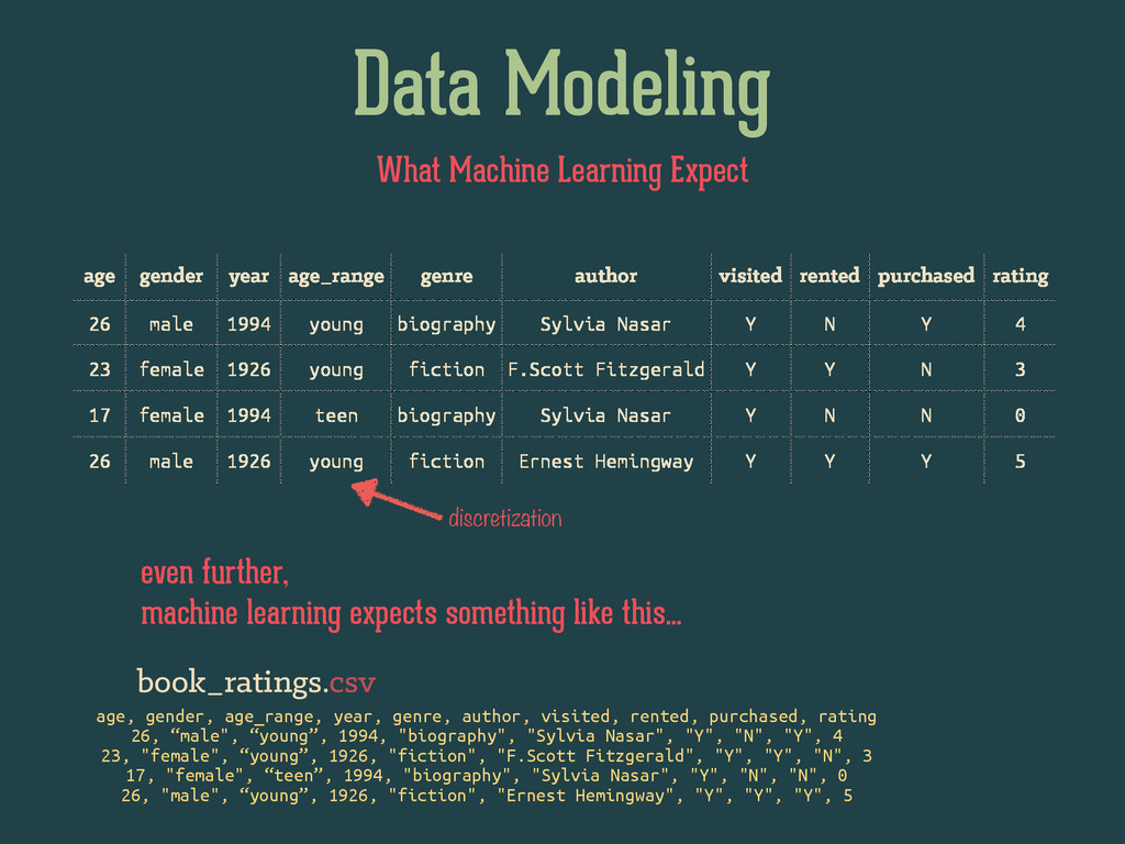
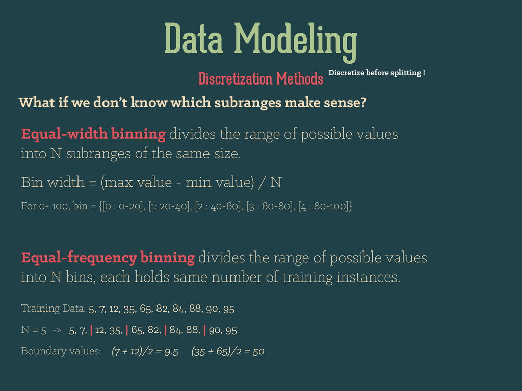
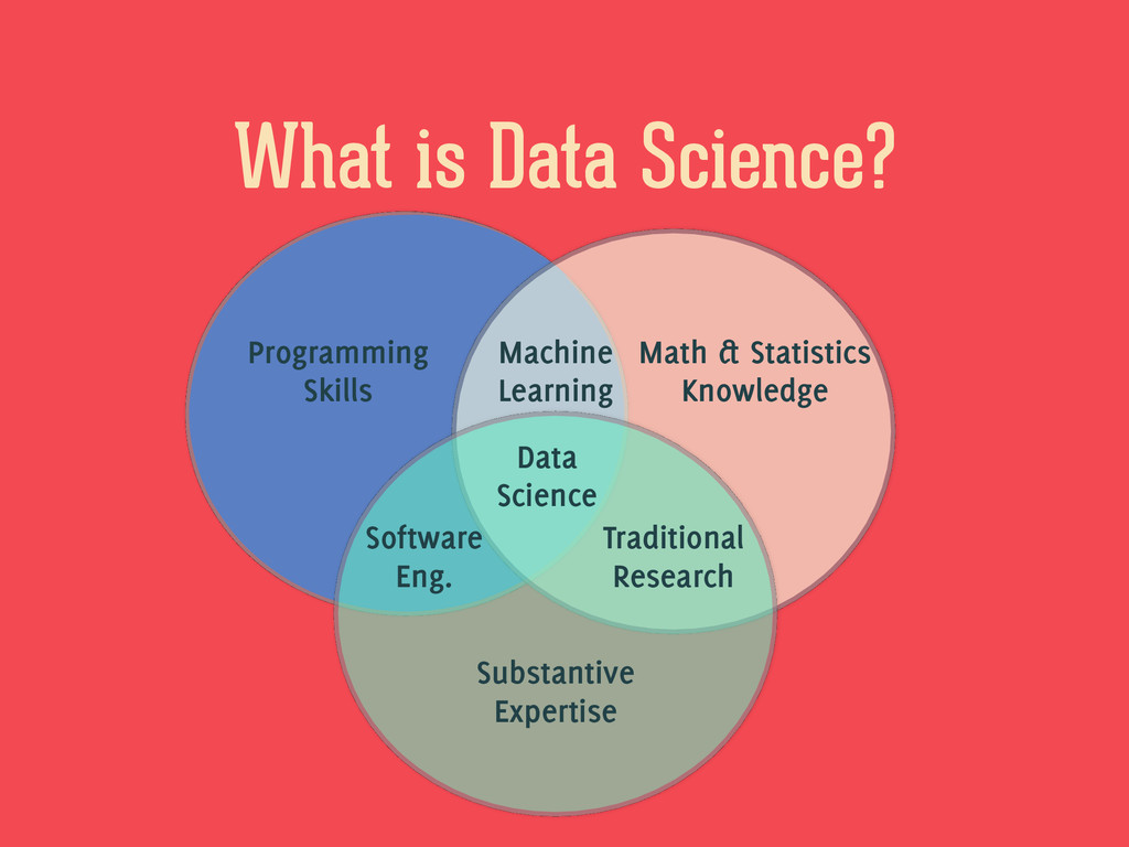
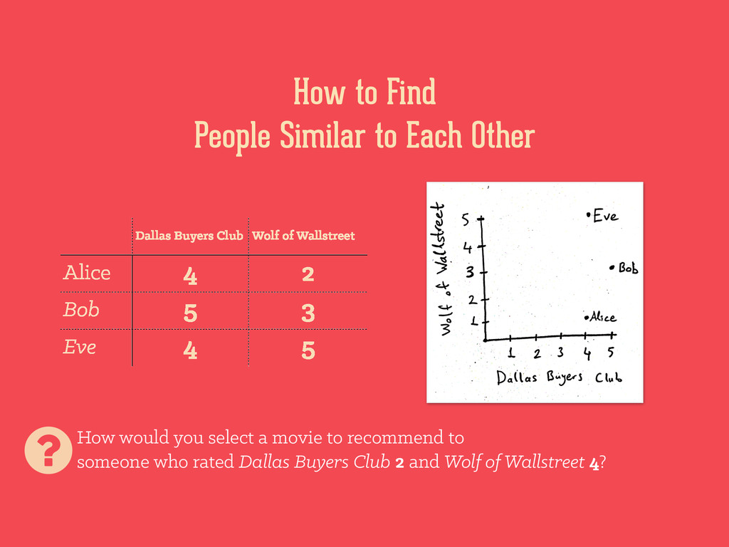
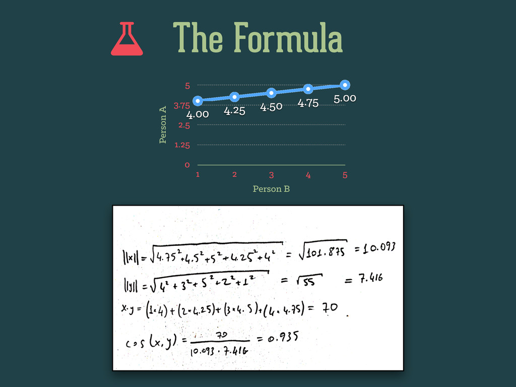
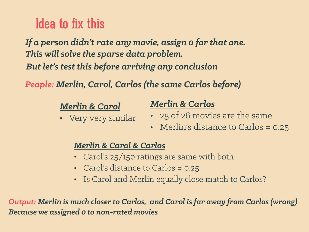
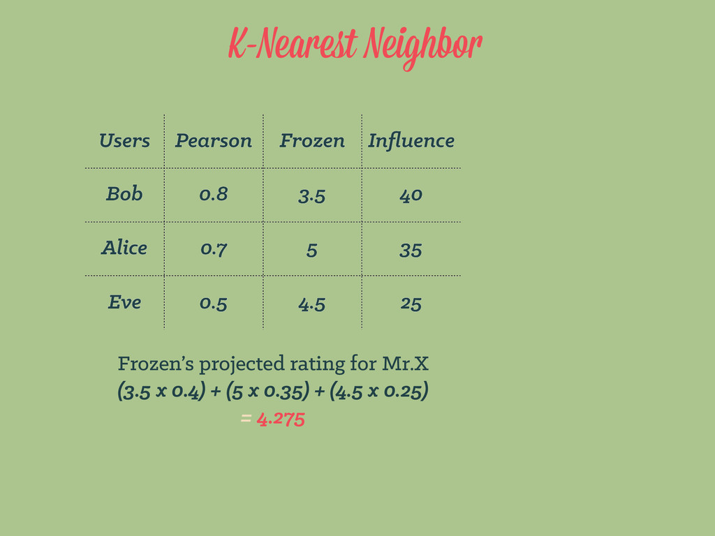
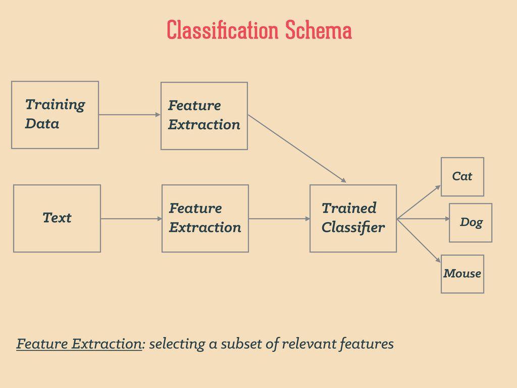
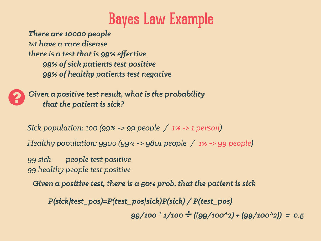
10. Data Modeling What Machine Learning Expect age gender year age_range genre author visited rented purchased rating 26 male 1994 young biography Sylvia Nasar Y N Y 4 23 female 1926 young fiction F.Scott Fitzgerald Y Y N 3 17 female 1994 teen biography Sylvia Nasar Y N N 0 26 male 1926 young fiction Ernest Hemingway Y Y Y 5 even further, machine learning expects something like this… age, gender, age_range, year, genre, author, visited, rented, purchased, rating 26, “male", “young”, 1994, "biography", "Sylvia Nasar", "Y", "N", "Y", 4 23, "female", “young”, 1926, "fiction", "F.Scott Fitzgerald", "Y", "Y", "N", 3 17, "female", “teen”, 1994, "biography", "Sylvia Nasar", "Y", "N", "N", 0 26, "male", “young”, 1926, "fiction", "Ernest Hemingway", "Y", "Y", "Y", 5 book_ratings.csv discretization
11. Data Modeling De-normalization: De-normalize your data! Multiple records " Single record Transform: Some algorithms only work with nominal values. Others only work with numbers. Discretization: Divide range of possible values into buckets. {[child : 0-12], [teen: 13-19], [young : 20-35], [middle : 36-59], [senior : 60+]} Dictionary Values: Like primary key columns in a database {[1 : Lion King], [2 : Toy Story], [3 : Finding Nemo]} Dividing up data: n% for training, 100-n% for test. Possible splits: 67/33, 80/20, 90/10
12. Data Modeling Discretization Methods What if we don’t know which subranges make sense? Equal-width binning divides the range of possible values into N subranges of the same size. Discretize before splitting ! Bin width = (max value - min value) / N For 0- 100, bin = {[0 : 0-20], [1: 20-40], [2 : 40-60], [3 : 60-80], [4 : 80-100]} Equal-frequency binning divides the range of possible values into N bins, each holds same number of training instances. Training Data: 5, 7, 12, 35, 65, 82, 84, 88, 90, 95 N = 5 -> 5, 7, | 12, 35, | 65, 82, | 84, 88, | 90, 95 Boundary values: (7 + 12)/2 = 9.5 (35 + 65)/2 = 50
13. Data Preparation Machines learn from data! ! Get the right data for the right problem ! Better data handling = more consistent results = more better ! ! Steps: Select Data Preprocess Data Transform Data
14. Data Preparation “more is better” ? Not necessarily always. ! Go for the right data for the right job. ! CONSIDER #: $ what data you actually need to address the problem ? $ what data you actually have ? $ what data is missing ? $ what data can be removed ? Step 1 → Select Data
15. Data Preparation Getting the selected data into a form that you can work ! Consider how you are going to use this data ! Formatting the data to fit your needs % & ' ! Cleaning is removal / fixing of missing or corrupted data −/+ ! Sampling is taking representative sample to faster prototyping ) Step 2 → Preprocess Data
16. Data Preparation The specific algorithm you are working with, and the knowledge of the problem domain will influence this step ! Scaling $, kg, sales volume… Scale for 0 and 1 (small / big ) * ! Decomposition Split out unnecessary details + ! Aggregation of features into a more meaningful one , Step 3 → Transform Data
17. What is Data Science? Substantive Expertise Programming Skills Software Eng. Math & Statistics Knowledge Traditional Research Machine Learning Data Science
18. • Do math • Write code • Ask questions Data Scientists do 3 things
19. Stack I Use Development Environment Version Control Deployment to Production (if it’s a web app) Programming + scikit-learn (numpy, scipy, matplotlib libraries)
20. Getting Started With Recommendation Systems Collaborative Filtering They like what you like, they also like these
21. How to Find People Similar to Each Other Dallas Buyers Club Wolf of Wallstreet Alice 4 2 Bob 5 3 Eve 4 5 How would you select a movie to recommend to someone who rated Dallas Buyers Club 2 and Wolf of Wallstreet 4? ?
22. You do this by computing distance Lets call Eve (x1, y1) and X (x2, y2) In a 2D world, each person is represented by (x, y) Eve’s distance to X is calculated by | x1 - x2| + | y1 - y2 | Distance from X Alice 4 Bob 4 Eve 3 We see that Eve is the closest match to X So we can look at Eve’s history and recommend her favorite movie to X . Manhattan Distance ?In which circumstance the Manhattan Distance would be the best choice? What would be its main benefit?
23. / Answer: It’s very fast to compute. If we were developing a social media application and were trying to find similar people to someone among millions of users, and running this computation against every users constantly, the speed would come in handy
24. Euclidean Distance Pythagorean Theorem: unlike the Manhattan Distance, we measure the bird’s-eye-view distance. a b c c=√a2+b2 And our formula is: √(x1-x2)2+(y1-y2)2 Distance from X Alice √ Bob √ Eve √ We see that Eve is the closest match again .
25. Let’s kick it up a notch Bob Alice Eve Merlin Carol Carlos Wendy Erin 12 Years a Slave 3.5 2 5 3 - - 5 3 Gravity 2 3.5 1 4 4 4.5 2 - Dallas Buyers Club - 4 1 4.5 1 4 - - Blue Jasmine 4.5 - 3 - 4 5 3 5 American Hustle 5 2 5 3 - 5 5 4 The Great Gatsby 1.5 3.5 1 4.5 - 4.5 4 2.5 Frozen 2.5 - - 4 4 4 5 3 Captain Phillips 2 3 - 2 1 4 - - Notice that some users didn’t rate some bands. We will compute the distance based on the number of bands they both reviewed. 0 Let’s compute difference between Bob and Alice
26. Alice & Bob Bob Alice Diff 12 Years a Slave 3.5 2 Gravity 2 3.5 Dallas Buyers Club - 4 Blue Jasmine 4.5 - American Hustle 5 2 The Great Gatsby 1.5 3.5 Frozen 2.5 - Captain Phillips 2 3 Manhattan Distance 9 Sum of Squares 18.5 Euclidean Distance 4.3 Manhattan Distance is the sum of differences (1.5 + 1.5 + 3 + 2 + 1) √(3.5 - 2)2 + (2 - 3.5)2 + (5 - 2)2 + (1.5 - 3.5)2 + (2 - 3)2 Euclidean Distance: ?Can you see a drawback with this process?
27. The Drawback − When we compute distance between Carol and Carlos, there were 5 dimensions Now, check out dimensions between Carol and Erin, there are 2 dimensions 2 Manhattan and Euclidian distances work best when there are no missing values √(4 - 5)2 + (4 - 3)2 = 1.41 √(4 - 4.5)2 + (1 - 4)2 + (4 - 5)2 + (4 - 4)2 + (1 - 4)2 = 4.39 Let’s compute distance between Carol and Erin Now, compute distance between Carol and Carlos " This situation puts our consistency in risk
28. The Formula 3 2 When we generalize Euclidian and Manhattan distances, we get Minkowski Distance Metric: " if r = 1, then it’s Manhattan Distance " if r = 2, then it’s Euclidian Distance " if r = ∞, then it’s Supremum Distance The bigger the r, the more a large difference in one dimension will influence the total difference
29. The Code 4 def nearest_neighbor(username, user_dict):! """! Input : a username that can be found on our ! dict, and our dict! Output: a sorted list of users based on their ! distance to username! Usage : nearest_neighbor('username', dictname)! """! distances = []! for user in user_dict:! if user != username:! distance = manhattan_distance(! user_dict[user], user_dict[! username])! #distance = minkowski_distance(! user_dict[user], user_dict[! username], 2)! # 1 -> Manhattan Distance! # 2 -> Euclidian Distance! distances.append((distance, user))! distances.sort() # sort based on min(distance)! return distances def manhattan_distance(user1, user2):! """ ! Input : 2 dict. elements! Output: manhattan distance value of two users! Usage : manhattan_distance(users['key1'], ! users['key2'])! """! distance = 0! has_common_ratings = False ! for key in user1:! if key in user2:! distance += abs(user1[key] - user2[key])! has_common_ratings = True! if has_common_ratings:! return distance! else:! return -1 # No ratings in common
30. Alice Carol Carlos 12 Years a Slave 2 - - Gravity 3.5 4 4.5 Dallas Buyers Club 4 1 4 Blue Jasmine - 4 5 American Hustle 2 - 5 The Great Gatsby 3.5 - 4.5 Frozen - 4 4 Captain Phillips 3 1 4 medium points extreme points very low or very high likes all. 4 or 5 every time ?How would you compare Carol to Carlos? Can we say Carol’s 4 = Carlos’ 5? 5 Can you see a drawback with all this processes?
31. Pearson Correlation Coefficient We measure the correlation between two variables It ranges between -1 (total mismatch) and 1 (total match) Person A 0 1.25 2.5 3.75 5 Person B 1 2 3 4 5 4.00 4.25 4.50 4.75 5.00 Person A 0 1.25 2.5 3.75 5 Person B 1 2 3 4 5 4.25 4.00 4.50 4.25 5.00 Person A 0 1.25 2.5 3.75 5 Person B 1 2 3 4 5 4.50 3.50 4.75 2.10 3.50
32. The Formula It’s a total match! 3
33. The Code 4 def pearson_corr(rating1, rating2):! sum_xy, sum_x, sum_y, sum_xsq, sum_ysq, n = 0, 0, 0, 0, 0, 0! for key in rating1:! if key in rating2:! n += 1! x = rating1[key]! y = rating2[key]! sum_xy += x * y! sum_x += x! sum_y += y! sum_xsq += pow(x, 2)! sum_ysq += pow(y, 2)! #denominator! denominator = sqrt(sum_xsq - pow(sum_x, 2) / n) * sqrt(sum_ysq - pow(sum_y, 2) / n)! if denominator == 0:! return 0! else:! return (sum_xy - (sum_x * sum_y) / n) / denominator!
34. Cosine Similarity There would be very little shared data among the huge dataset But we don’t want to use shared zeros. Number of Plays Alanis Morissette Ironic B.o.B So Good Coldplay Magic Bob 10 5 32 Alice 15 25 1 Eve 12 36 27 Think word frequency in a book Measure of similarity between two vectors of an inner product space that measures the cosine of the angle between them (in our case, # of plays!) One of the reasons for the popularity of Cosine similarity is that it is very efficient to evaluate, especially for sparse vectors, as only the non-zero dimensions need to be considered.
35. The Formula 3
36. The Formula 3 Person A 0 1.25 2.5 3.75 5 Person B 1 2 3 4 5 4.00 4.25 4.50 4.75 5.00
37. The Code 4 import math! ! def cosine_similarity(v1,v2):! sumxx, sumxy, sumyy = 0, 0, 0! for i in range(len(v1)):! x = v1[i]; y = v2[i]! sumxx += x*x! sumyy += y*y! sumxy += x*y! return sumxy/math.sqrt(sumxx*sumyy)!
38. ? Question: Which one should we chose? In what circumstances?
39. / Answer: • Use Manhattan/Euclidean distances if your data is dense (No zero valued attributes) • Use Pearson Correlation Coefficient if your data is using different scales. • Use Cosine Similarity if your data is sparse
40. Case #1 People: Bob, Alice, Carlos 6 Movie Rating System: Bob & Alice • 20 movies in common • Diff. in ratings = 0.5 (in 1-5 scale) • Manhattan(Bob, Alice) : 20 x 0.5 = 10 • Euclidean(Bob, Alice) : √0.52 x 20 = 2.36 Alice & Carlos • 1 movie in common • Diff. in ratings = 2 (in 1-5 scale) • Manhattan(Alice, Carlos) : 1 x 2 = 2 • Euclidean(Bob, Alice) : √22 = 2 Output: Carlos is a better match to Alice (which is wrong)
41. Idea to fix this If a person didn’t rate any movie, assign 0 for that one. This will solve the sparse data problem. Merlin & Carlos • 25 of 26 movies are the same • Merlin’s distance to Carlos = 0.25 Output: Merlin is much closer to Carlos, and Carol is far away from Carlos (wrong) Because we assigned 0 to non-rated movies People: Merlin, Carol, Carlos (the same Carlos before) Merlin & Carol • Very very similar Merlin & Carol & Carlos • Carol’s 25/150 ratings are same with both • Carol’s distance to Carlos = 0.25 • Is Carol and Merlin equally close match to Carlos? But let’s test this before arriving any conclusion
42. Take-Home Lesson 0 values dominate the measure in distances. ! If data is not dense, making it sparse by modification will create another problems when solving one. ! If data is sparse, using cosine similarity will be much better for us.
43. Case #2 People: Bob, Carol, Bob’s wife Alice 6 Book Rating System: Bob & Carol • Has gave 5 stars to same books (Game of Thrones, Lord of the Rings, Dune) • Bob’s wife wrote a book about botany • Bob gave this book 5 stars because the author is his wife • Since Bob is the closest person to Carol, recommend this botany book to Carol Why?: Because we are still recommending by looking at 1-to-1 relationships ?What can we do?
44. K-Nearest Neighbor We use K most similar people to determine recommendations What should K be? Well, it’s up to you, and application Recommendation to Mr.X with kNN where k =3 Users Pearson Bob 0.8 Alice 0.7 Eve 0.5 0.7 + 0.8 + 0.5 = 2.0 Influence Coeff. 25% 35% 40% Bob Alice Eve Users Frozen Bob 3.5 Alice 5 Eve 4.5
45. K-Nearest Neighbor Users Pearson Frozen Influence Bob 0.8 3.5 40 Alice 0.7 5 35 Eve 0.5 4.5 25 Frozen’s projected rating for Mr.X (3.5 x 0.4) + (5 x 0.35) + (4.5 x 0.25) = 4.275
46. Classification Drawback with Collaborative Filtering: Tends to recommend already popular items. Brand new items will never be found and rated easily, thus never recommended and they will be thrown to side. Why not classify them? That way, we can find similar items, not only similar users.
47. Importance of Selecting Appropriate Values Y axis Genre Value Country 1 Jazz 2 Rock 3 Soul 4 Rap 5 X axis Mood Value Melancholy 1 Joyful 2 Passion 3 Angry 4 Other 5 James Blunt - You’re Beautiful = (1,3) Song A = (1,2) Song B = (4,4) Song C = (4,2) Song A is the closest to our sample. With that logic, we are saying that Jazz is closer to Rock than it is to Soul, and Melancholy is closer to Joy than it is to Angry It’s a big mistake and won’t gone even if we change the order
48. Importance of Selecting Appropriate Values Why not classify put them in their own scales? Melancholic? How melancholic? Rock? What is the coefficient? ! E.g : Country(5/5), Soul(3/5), Rock(1/5) and Joy(3/5) Passion(3/5) ! A nice example (all of them has their own scales): ! • Amount of piano • Amount of vocals • Driving beat • Blues Influence • Presence of dirty electric guitar • Presence of backup vocals • Rap Influence ! Once we define our values and scales, it’s just a matter of applying Nearest Neighbor algorithm /
49. Classification Schema Text Feature Extraction Trained Classifier Training Data Feature Extraction Cat Dog Mouse Feature Extraction: selecting a subset of relevant features
50. Probability P(A) is the probability that A is true Axioms of Probability P(True) = 1 ! P(False) = 0 ! 0 ≤ P(A) ≤ 1 ! P(A or B) = P(A) + P(B) - P(A and B) P(A) P(B) P(A and B)
51. Naïve Bayes Nearest Neighbor: Lazy Learner When we give them a set of data, they save the set for that instance. Each time it classifies an instance, it goes through the whole training set. 100,000 music tracks -> goes through all of them each time it classifies an instance Bayesian Methods: Eager Learner Immediately analyze data and build model When classifying an instance, it uses this internal model. Probabilistic classifications and faster classification are main benefits of the Bayesian methods
52. Bayes Law p(A|B)p(B) p(B|A) = —————— p(A) Corner stone of all Bayesian methods You can calculate the probability of event B if A. If you already knew the probability of A given B and B and A individually Probability of event B if A what is the probability of event B is occurring, if A is occurred
53. Bayes Law Example There are 10000 people %1 have a rare disease there is a test that is 99% effective 99% of sick patients test positive 99% of healthy patients test negative ! Given a positive test result, what is the probability that the patient is sick? ? Sick population: 100 (99% -> 99 people / 1% -> 1 person) Healthy population: 9900 (99% -> 9801 people / 1% -> 99 people) 99 sick people test positive 99 healthy people test positive Given a positive test, there is a 50% prob. that the patient is sick P(sick|test_pos)=P(test_pos|sick)P(sick) / P(test_pos) 99/100 * 1/100 ÷ ((99/100^2) + (99/100^2)) = 0.5
54. Unstructured Text Classification with Naïve Bayes Check the code!
55. Linear Regression Explains the relationship between a dependent variable and one or more explanatory variables. ! This is a tool to show the relationship between the inputs and outputs of a system. ! Does any change in x, causes something in y? ! Commonly used in customer satisfaction researches. ! More efficient with short term trend data. ! Check the code!
56. scikit-learn Statistical Learning with scikit-learn (Also the SVM) A simple example: Iris Dataset >>> from sklearn import datasets >>> iris = datasets.load_iris() >>> data = iris.data >>> data.shape (150, 4) It is made of 150 observations of irises, each described by 4 features: their sepal and petal length and width When the data is not initially in the (n_samples, n_features) shape, it needs to be preprocessed in order to by used by scikit 2
57. >>> from sklearn import datasets >>> from sklearn import datasets, svm, metrics >>> digits = datasets.load_digits() >>> for index, (image, label) in enumerate(zip(digits.images, digits.target)[:4]): pl.subplot(2, 4, index + 1) pl.axis('off') pl.imshow(image, cmap=pl.cm.gray_r, interpolation='nearest') pl.title('Training: %i' % label) >>> # To apply an classifier on this data, we need to flatten the image >>> # to turn the data in a (samples, feature) matrix >>> n_samples = len(digits.images) >>> data = digits.images.reshape((n_samples, -1)) ! >>> # support vector classifier >>> classifier = svm.SVC(gamma=0.001) ! >>> # We learn the digits on the first half of the digits >>> classifier.fit(data[:n_samples / 2], digits.target[:n_samples / 2]) ! >>> # Now predict the value of the digit on the second half: >>> expected = digits.target[n_samples / 2:] >>> predicted = classifier.predict(data[n_samples / 2:])
58. >>> for index, (image, prediction) in enumerate( zip(digits.images[n_samples / 2:], predicted)[:4]): pl.subplot(2, 4, index + 5) pl.subplot(2, 4, index + 5) pl.axis('off') pl.imshow(image, cmap=pl.cm.gray_r, interpolation='nearest') pl.title('Prediction: %i' % prediction) >>> pl.show()
59. THANK YOU