Analytics in AWS - Boston AWS, June 2013

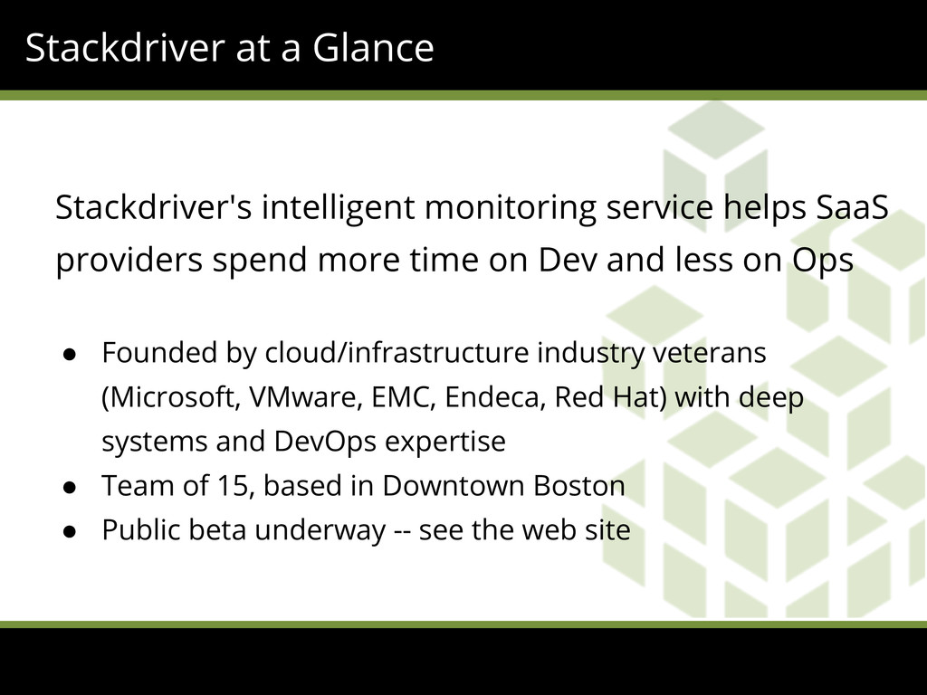
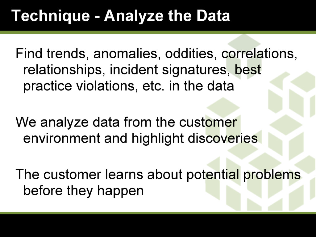
In his presentation (first delivered at the Boston AWS meetup on June 10th, 2013), Stackdriver's Patrick Eaton describes the role of analytics in the Stackdriver Intelligent Monitoring service. He highlights three techniques that we use and share a little bit about the tools and algorithms behind the analysis

Transcript

1. Analytics in AWS Patrick Eaton, PhD patrick@stackdriver.com @PatrickREaton
2. Stackdriver at a Glance Stackdriver's intelligent monitoring service helps SaaS providers spend more time on Dev and less on Ops • Founded by cloud/infrastructure industry veterans (Microsoft, VMware, EMC, Endeca, Red Hat) with deep systems and DevOps expertise • Team of 15, based in Downtown Boston • Public beta underway -- see the web site
3. Analytics at Stackdriver Goal: Deliver more value for less effort Examples: • Monitor and report on infrastructure in terms that makes sense to your team • Detect how pieces of the infrastructure relate • Display lots of data at one time • Suggest policies to alert you of possible problems • Identify unusual application behavior This talk: three broad analytics techniques and examples
4. Technique: Mine the Metadata • AWS provides heaps of metadata about your infrastructure • Metadata is accessible via Amazon's APIs • Use it! Simple analysis of the metadata can produce big wins
5. Using Metadata - Identify App Groups • We make suggestions based on instance names, tags, security groups, etc. • Customer gets more relevant monitoring
6. Using Metadata - Find Relationships • We make explicit the relationships in the customers infrastructure ◦ load balancers and backing instances ◦ instances and security groups ◦ volumes and their host ◦ snapshots and their volumes • Customer sees an architectural view that matches their mental model
7. Technique - Pre-compute Summarizations • Modern UIs are data rich • Data summarization is key for effectively presentation and UI performance • Identify commonly-used summarizations and pre- compute them (outside the critical path)
8. Summarizing - Roll-up Across Time We summarize data for a resource across time • Compute roll-ups for various functions: avg, max, percentile, etc. Customer can see historical trends quickly 30x Time 30min roll-up
9. Summarizing - Roll-up Across Resources We summarize behavior of multiple resources • Compute roll-ups for various functions: avg, max, percentile, etc. Customer can view cluster performance at a glance 15 resources
10. Tools for Summarization Tools • Hadoop and AWS Elastic Map/Reduce (EMR) • Python and mrjob ◦ https://github.com/Yelp/mrjob • Data from S3 archives; data to Cassandra Usage • EMR clusters of 14 c1.mediums • Start jobs every 6 hours
11. mrjob Word Count Example from mrjob.job import MRJob import re WORD_RE = re.compile(r"[\w']+") class MRWordFreqCount(MRJob): def mapper(self, _, line): for word in WORD_RE.findall(line): yield (word.lower(), 1) def combiner(self, word, counts): yield (word, sum(counts)) def reducer(self, word, counts): yield (word, sum(counts)) if __name__ == '__main__': MRWordFreqCount.run() Define map() and reduce() functions in standard Python Python generators pass data back to Hadoop mrjob handles set-up and configuration of job $ python mrjob_wc.py readme.txt > counts # local $ python mrjob_wc.py readme.txt -r emr > counts # EMR $ python mrjob_wc.py readme.txt -r hadoop > counts # Hadoop
12. Summarization Algorithm • Phase 0 ◦ Map ▪ Read archives from s3 ▪ Route data point to a time bucket for aggregation • key = resource::metric::time::granularity ◦ Reduce ▪ Aggregate data into a single data point ▪ We compute 8 functions (min, max, avg, med...) • Phase 1 ◦ Map ▪ Route aggregated point to a data series • key = resource::metric:granularity::aggr_fn ◦ Reduce ▪ Write series of data to Cassandra
13. Summarization Algorithm Illustrated t t + δ t + 2δ t+5+δ t + 5 t + 3δ Raw Data 5-Minute 15-Minute min max avg min max avg min max avg ... ... ... min min min max max max avg avg avg min min min max max max avg avg avg Map-0 Red-0 Map-1
14. Technique - Analyze the Data Find trends, anomalies, oddities, correlations, relationships, incident signatures, best practice violations, etc. in the data We analyze data from the customer environment and highlight discoveries The customer learns about potential problems before they happen
15. Analyzing - Suggest Alert Policies The product supports threshold-based alerts. We analyze historical data and suggest policies to catch future issues. Approach: analyze data series looking for typically consistent performance with statistically significant outliers • Use mrjob in local mode - easy programming model for smaller data sets
16. Analyzing - Identify Anomalies A more sophisticated version of the previous Currently using R for much of this analysis Using rpy2 to translate to/from Python (http://rpy.sourceforge.net/rpy2.html)
17. Example of rpy2 import rpy2.robjects as robjects robjects.r(''' find_decomposition <- function(data_series) { ts <- ts(data_series, start=c(1, 1), frequency=12) decomp <- decompose(ts, type="additive") } ''') def decompose(df, series): decomp_components = ['seasonal', 'trend', 'random'] decompose_fn = robjects.r['find_decomposition'] return decompose_fn(series)
18. Thank you! Yes, we are hiring! Patrick Eaton - patrick@stackdriver.com - @PatrickREaton