σ-semistability of quiver reps generalizes nc-nonsingularity of linear matrices, membership of Brascamp-Lieb polytopes, etc. • There are nice connections to network/submodular flow! 2 / 34
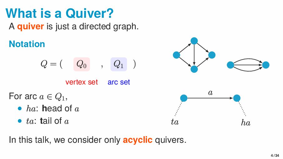
graph. Notation Q = ( Q0 vertex set , Q1 arc set ) For arc a ∈ Q1 , • ha: head of a • ta: tail of a a ta ha In this talk, we consider only acyclic quivers. 4 / 34
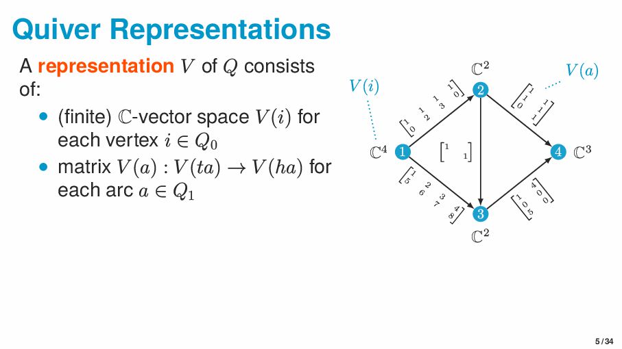
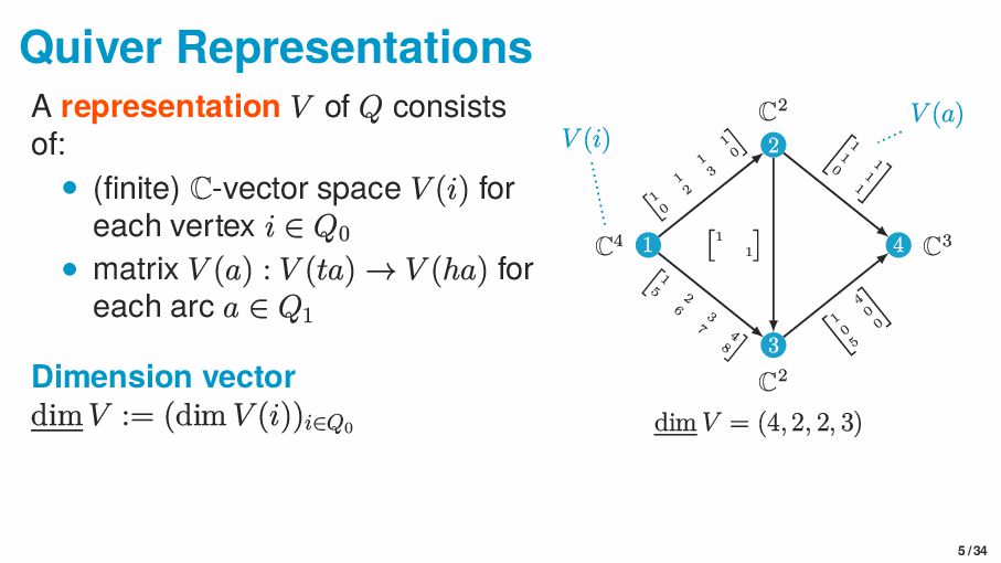
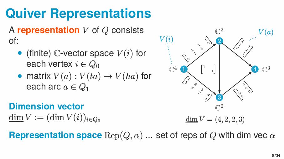
(finite) C-vector space V (i) for each vertex i ∈ Q0 • matrix V (a) : V (ta) → V (ha) for each arc a ∈ Q1 Dimension vector dim V := (dim V (i))i∈Q0 1 2 3 4 1 1 1 1 0 2 3 0 1 2 3 4 5 6 7 8 1 1 1 4 0 0 5 0 1 1 1 1 0 1 C4 C2 C2 C3 V (i) V (a) dim V = (4, 2, 2, 3) 5 / 34
(finite) C-vector space V (i) for each vertex i ∈ Q0 • matrix V (a) : V (ta) → V (ha) for each arc a ∈ Q1 Dimension vector dim V := (dim V (i))i∈Q0 1 2 3 4 1 1 1 1 0 2 3 0 1 2 3 4 5 6 7 8 1 1 1 4 0 0 5 0 1 1 1 1 0 1 C4 C2 C2 C3 V (i) V (a) dim V = (4, 2, 2, 3) Representation space Rep(Q, α) ... set of reps of Q with dim vec α 5 / 34
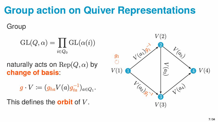
GL(α(i)) naturally acts on Rep(Q, α) by change of basis: g · V := (gha V (a)g−1 ta )a∈Q1 . This defines the orbit of V . 1 2 3 4 V (a1 ) V (a 2 ) V (a3 ) V (a4 ) V (a 5 ) V (1) V (2) V (3) V (4) g1 ⟳ g2 ⟳ g4 ⟳ ⟳ g3 7 / 34
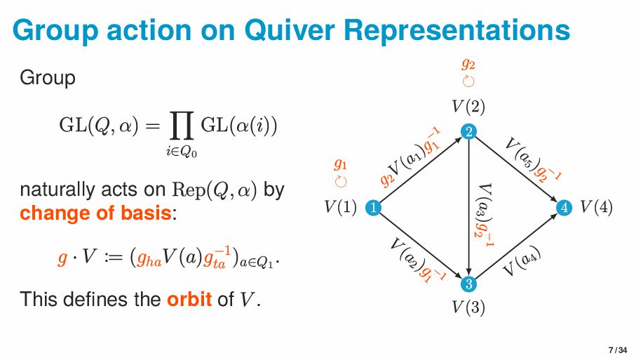
GL(α(i)) naturally acts on Rep(Q, α) by change of basis: g · V := (gha V (a)g−1 ta )a∈Q1 . This defines the orbit of V . 1 2 3 4 V (a1 )g − 1 1 V (a 2 )g − 1 1 V (a3 ) V (a4 ) V (a 5 ) V (1) V (2) V (3) V (4) g1 ⟳ g2 ⟳ g4 ⟳ ⟳ g3 7 / 34
GL(α(i)) naturally acts on Rep(Q, α) by change of basis: g · V := (gha V (a)g−1 ta )a∈Q1 . This defines the orbit of V . 1 2 3 4 g2 V (a1 )g − 1 1 V (a 2 )g − 1 1 V (a3 )g−1 2 V (a4 ) V (a 5 )g − 1 2 V (1) V (2) V (3) V (4) g1 ⟳ g2 ⟳ g4 ⟳ ⟳ g3 7 / 34
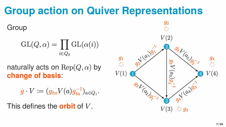
GL(α(i)) naturally acts on Rep(Q, α) by change of basis: g · V := (gha V (a)g−1 ta )a∈Q1 . This defines the orbit of V . 1 2 3 4 g2 V (a1 )g − 1 1 g 3 V (a 2 )g − 1 1 g3 V (a3 )g−1 2 g4 V (a4 )g − 1 3 g 4 V (a 5 )g − 1 2 V (1) V (2) V (3) V (4) g1 ⟳ g2 ⟳ g4 ⟳ ⟳ g3 7 / 34
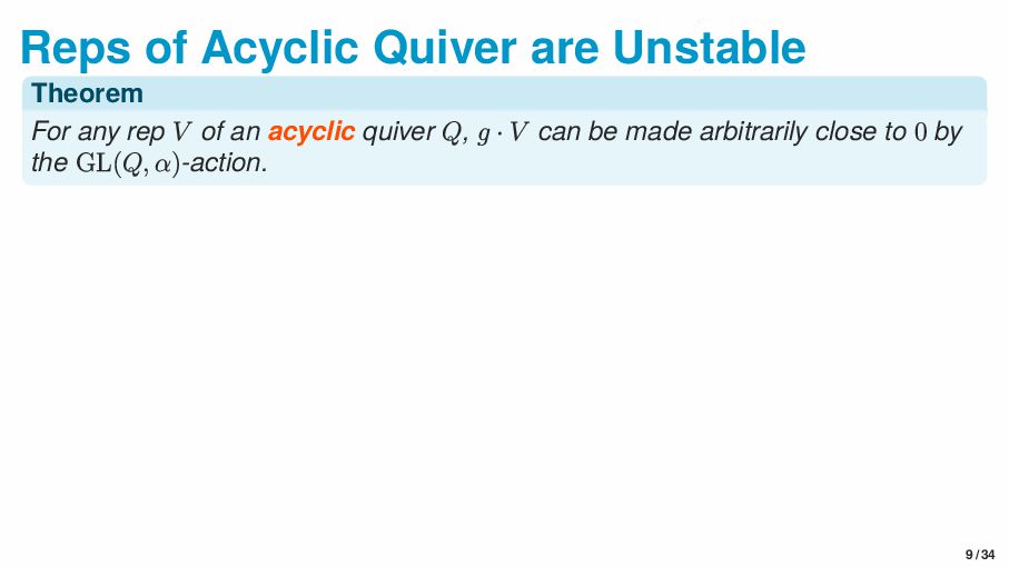
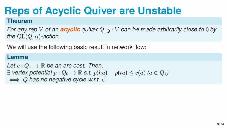
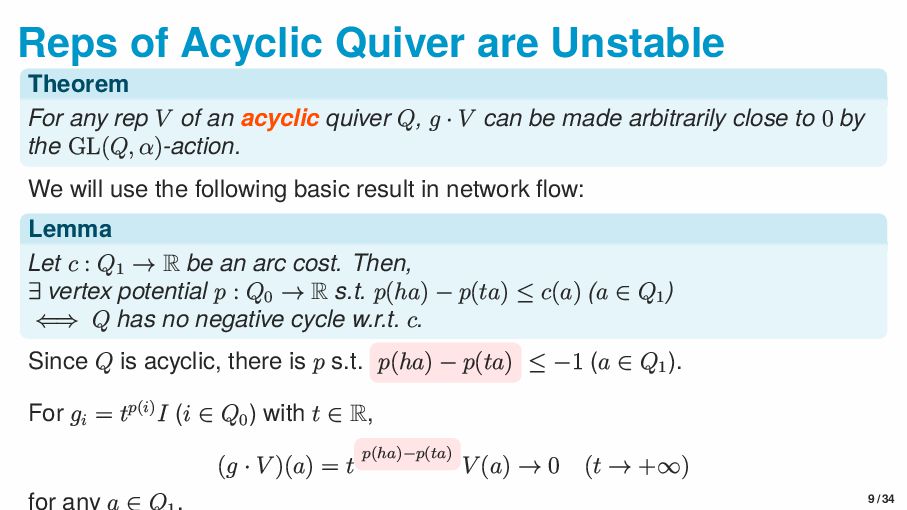
V of an acyclic quiver Q, g · V can be made arbitrarily close to 0 by the GL(Q, α)-action. We will use the following basic result in network flow: Lemma Let c : Q1 → R be an arc cost. Then, ∃ vertex potential p : Q0 → R s.t. p(ha) − p(ta) ≤ c(a) (a ∈ Q1 ) ⇐⇒ Q has no negative cycle w.r.t. c. 9 / 34
V of an acyclic quiver Q, g · V can be made arbitrarily close to 0 by the GL(Q, α)-action. We will use the following basic result in network flow: Lemma Let c : Q1 → R be an arc cost. Then, ∃ vertex potential p : Q0 → R s.t. p(ha) − p(ta) ≤ c(a) (a ∈ Q1 ) ⇐⇒ Q has no negative cycle w.r.t. c. Since Q is acyclic, there is p s.t. p(ha) − p(ta) ≤ −1 (a ∈ Q1 ). For gi = tp(i)I (i ∈ Q0 ) with t ∈ R, (g · V )(a) = t p(ha)−p(ta) V (a) → 0 (t → +∞) 9 / 34
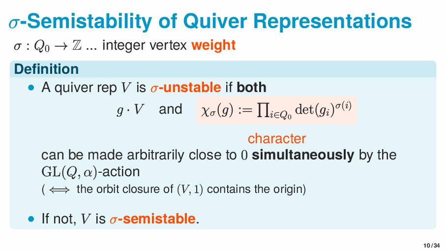
integer vertex weight Definition • A quiver rep V is σ-unstable if both g · V and χσ (g) := i∈Q0 det(gi )σ(i) character can be made arbitrarily close to 0 simultaneously by the GL(Q, α)-action ( ⇐⇒ the orbit closure of (V, 1) contains the origin) • If not, V is σ-semistable. 10 / 34
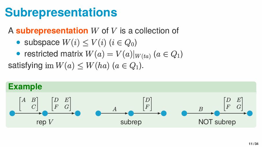
• subspace W(i) ≤ V (i) (i ∈ Q0 ) • restricted matrix W(a) = V (a)|W(ta) (a ∈ Q1 ) satisfying im W(a) ≤ W(ha) (a ∈ Q1 ). Example A B C D E F G rep V A D F subrep B D E F G NOT subrep 11 / 34
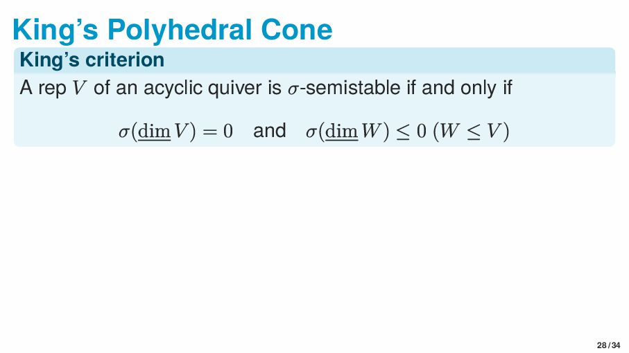
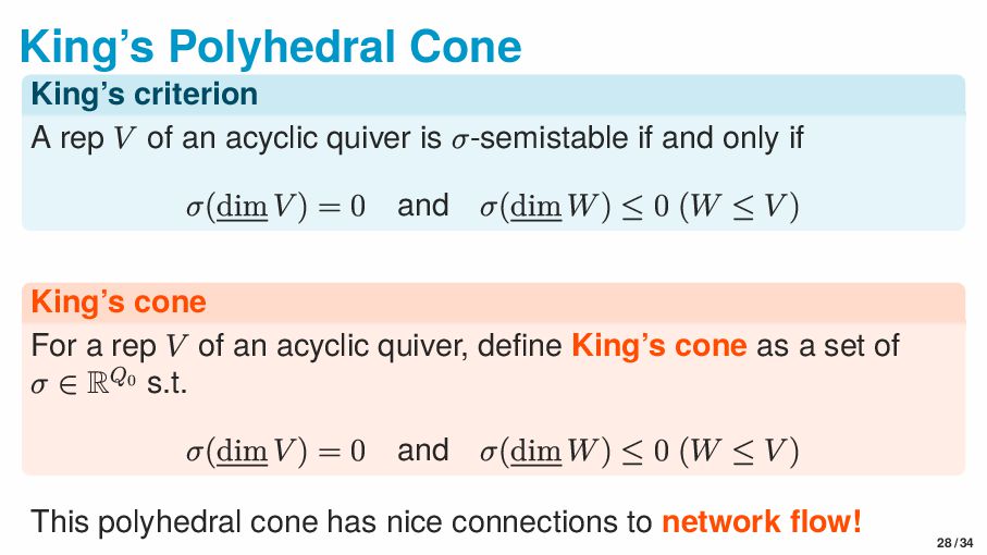
linear system: King’s criterion A rep V of an acyclic quiver is σ-semistable ⇐⇒ σ(dim V ) = 0 and σ(dim W) ≤ 0 (W ≤ V ) σ(α) := i∈Q0 σ(i)α(i) W ≤ V means W is a subrep of V 12 / 34
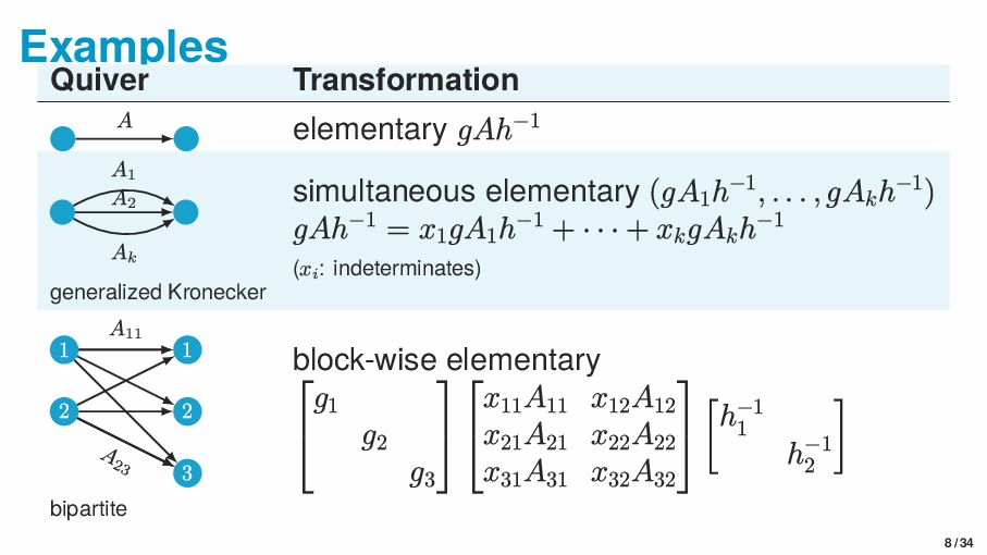
linear system: King’s criterion A rep V of an acyclic quiver is σ-semistable ⇐⇒ σ(dim V ) = 0 and σ(dim W) ≤ 0 (W ≤ V ) σ(α) := i∈Q0 σ(i)α(i) W ≤ V means W is a subrep of V Example V : A1 . . . Ak , dim V = (n, n), σ = (1, −1) ←→ linear matrix A = k a=1 xa Aa dim W1 − dim W2 ≤ 0 (W1 ≤ Cn, k Aa W1 ≤ W2 ) 12 / 34
linear system: King’s criterion A rep V of an acyclic quiver is σ-semistable ⇐⇒ σ(dim V ) = 0 and σ(dim W) ≤ 0 (W ≤ V ) σ(α) := i∈Q0 σ(i)α(i) W ≤ V means W is a subrep of V Example V : A1 . . . Ak , dim V = (n, n), σ = (1, −1) ←→ linear matrix A = k a=1 xa Aa dim W − dim k Aa W ≤ 0 (W ≤ Cn) Nc-nonsingularity of A 12 / 34
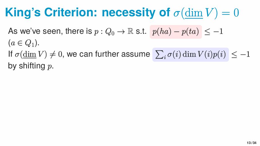
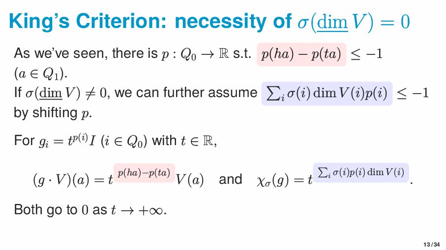
we’ve seen, there is p : Q0 → R s.t. p(ha) − p(ta) ≤ −1 (a ∈ Q1 ). If σ(dim V ) ̸= 0, we can further assume i σ(i) dim V (i)p(i) ≤ −1 by shifting p. 13 / 34
we’ve seen, there is p : Q0 → R s.t. p(ha) − p(ta) ≤ −1 (a ∈ Q1 ). If σ(dim V ) ̸= 0, we can further assume i σ(i) dim V (i)p(i) ≤ −1 by shifting p. For gi = tp(i)I (i ∈ Q0 ) with t ∈ R, (g · V )(a) = t p(ha)−p(ta) V (a) and χσ (g) = t i σ(i)p(i) dim V (i) . Both go to 0 as t → +∞. 13 / 34
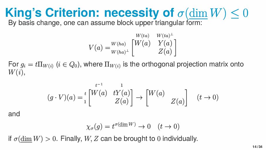
change, one can assume block upper triangular form: V (a) = W(ta) W(ta)⊥ W(ha) W(a) Y (a) W(ha)⊥ Z(a) For gi = tΠW(i) (i ∈ Q0 ), where ΠW(i) is the orthogonal projection matrix onto W(i), (g · V )(a) = t−1 1 t W(a) tY (a) 1 Z(a) → W(a) Z(a) (t → 0) and χσ (g) = tσ(dim W) → 0 (t → 0) if σ(dim W) > 0. Finally, W, Z can be brought to 0 individually. 14 / 34
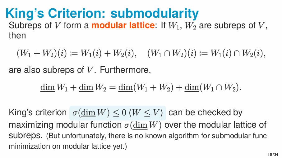
If W1 , W2 are subreps of V , then (W1 + W2 )(i) := W1 (i) + W2 (i), (W1 ∩ W2 )(i) := W1 (i) ∩ W2 (i), are also subreps of V . Furthermore, dim W1 + dim W2 = dim(W1 + W2 ) + dim(W1 ∩ W2 ). King’s criterion σ(dim W) ≤ 0 (W ≤ V ) can be checked by maximizing modular function σ(dim W) over the modular lattice of subreps. (But unfortunately, there is no known algorithm for submodular func minimization on modular lattice yet.) 15 / 34
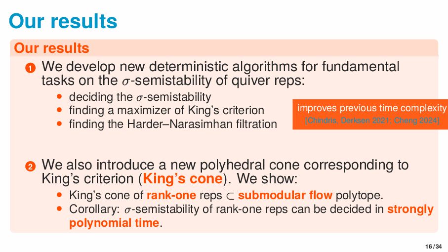
for fundamental tasks on the σ-semistability of quiver reps: • deciding the σ-semistability • finding a maximizer of King’s criterion • finding the Harder–Narasimhan filtration improves previous time complexity [Chindris, Derksen 2021; Cheng 2024] 2 We also introduce a new polyhedral cone corresponding to King’s criterion (King’s cone). We show: • King’s cone of rank-one reps ⊂ submodular flow polytope. • Corollary: σ-semistability of rank-one reps can be decided in strongly polynomial time. 16 / 34
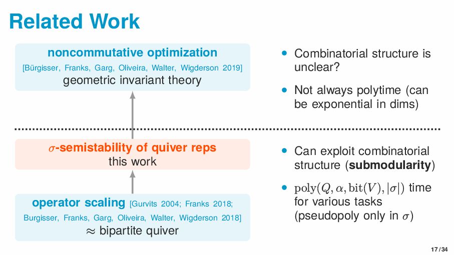
Garg, Oliveira, Walter, Wigderson 2018] ≈ bipartite quiver σ-semistability of quiver reps this work noncommutative optimization [Bürgisser, Franks, Garg, Oliveira, Walter, Wigderson 2019] geometric invariant theory • Combinatorial structure is unclear? • Not always polytime (can be exponential in dims) • Can exploit combinatorial structure (submodularity) • poly(Q, α, bit(V ), |σ|) time for various tasks (pseudopoly only in σ) 17 / 34
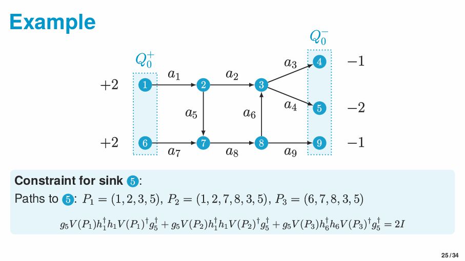
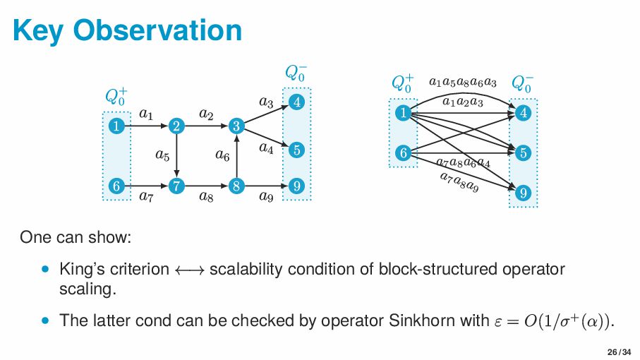
0 1 2 3 4 5 6 7 8 9 a1 a2 a3 a4 a7 a8 a9 a5 a6 Q+ 0 Q− 0 1 6 4 5 9 a1 a2 a3 a1 a5 a8 a6 a3 a7 a8 a6 a4 a 7a 8a 9 For a path P = a1 a2 · · · ak in Q, define V (P) := V (ak ) · · · V (a2 )V (a1 ). V induces a rep V ′ on the bipartite quiver by assigning V (P) to each path P. 19 / 34
0 1 2 3 4 5 6 7 8 9 a1 a2 a3 a4 a7 a8 a9 a5 a6 Q+ 0 Q− 0 1 6 4 5 9 a1 a2 a3 a1 a5 a8 a6 a3 a7 a8 a6 a4 a 7a 8a 9 For a path P = a1 a2 · · · ak in Q, define V (P) := V (ak ) · · · V (a2 )V (a1 ). V induces a rep V ′ on the bipartite quiver by assigning V (P) to each path P. Theorem ([Derksen, Makam 2017; Huszar 2021]) V is σ-semistable ⇐⇒ V ′ is σ′-semistable, where σ′ is the restriction of σ to Q+ 0 ˙ ∪Q− 0 19 / 34
1 Compute the Cholesky decomposition CC† = k i=1 ˜ Ai ˜ A† i . Set g = Diag(p)1/2C−1 and ˜ Ai ← g ˜ Ai . (left normalization) 2 Compute the Cholesky decomposition CC† = k i=1 ˜ A† i ˜ Ai . Set h = Diag(q)1/2C−1 and ˜ Ai ← ˜ Ai h†. (right normalization) 21 / 34
1 Compute the Cholesky decomposition CC† = k i=1 ˜ Ai ˜ A† i . Set g = Diag(p)1/2C−1 and ˜ Ai ← g ˜ Ai . (left normalization) 2 Compute the Cholesky decomposition CC† = k i=1 ˜ A† i ˜ Ai . Set h = Diag(q)1/2C−1 and ˜ Ai ← ˜ Ai h†. (right normalization) Theorem ([Burgisser, Franks, Garg, Oliveira, Walter, Wigderson 2018]) If a solution exists, then the operator Sinkhorn iteration converges to a solution in O(ε−2(b + N log(ℓN))) iterations (b: maximum bit length of Ai , N := max{m, n}, ℓ: the smallest positive integer s.t. ℓ(p, q) is integral). 21 / 34
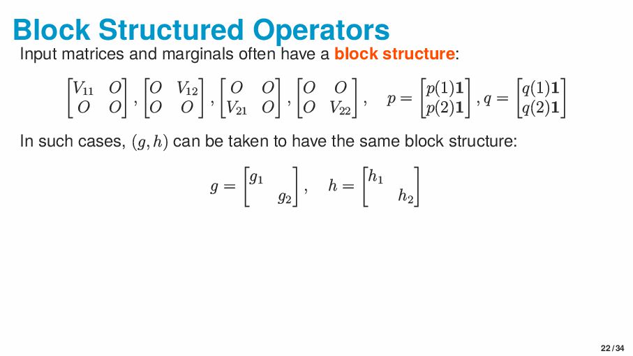
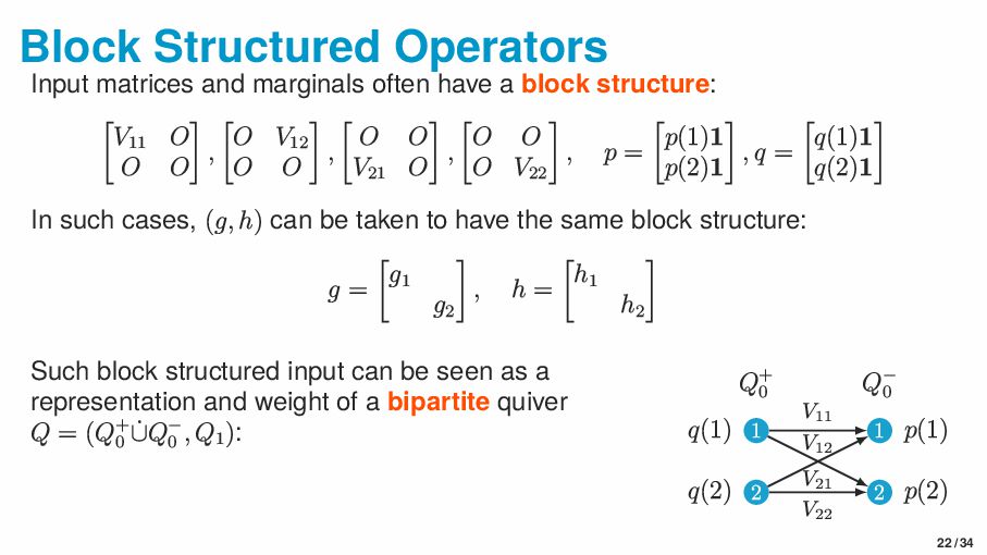
block structure: V11 O O O , O V12 O O , O O V21 O , O O O V22 , p = p(1)1 p(2)1 , q = q(1)1 q(2)1 In such cases, (g, h) can be taken to have the same block structure: g = g1 g2 , h = h1 h2 22 / 34
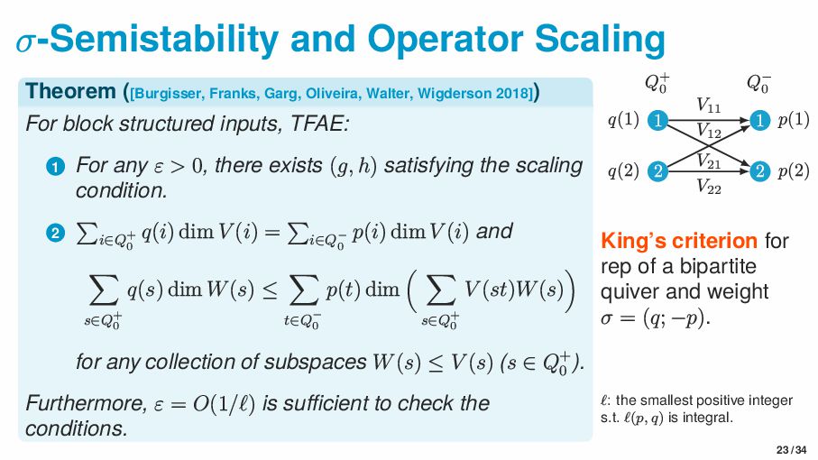
block structure: V11 O O O , O V12 O O , O O V21 O , O O O V22 , p = p(1)1 p(2)1 , q = q(1)1 q(2)1 In such cases, (g, h) can be taken to have the same block structure: g = g1 g2 , h = h1 h2 Such block structured input can be seen as a representation and weight of a bipartite quiver Q = (Q+ 0 ˙ ∪Q− 0 , Q1 ): 1 2 1 2 q(1) q(2) p(1) p(2) Q+ 0 Q− 0 V11 V12 V21 V22 22 / 34
Wigderson 2018]) For block structured inputs, TFAE: 1 For any ε > 0, there exists (g, h) satisfying the scaling condition. 2 i∈Q+ 0 q(i) dim V (i) = i∈Q− 0 p(i) dim V (i) and s∈Q+ 0 q(s) dim W(s) ≤ t∈Q− 0 p(t) dim s∈Q+ 0 V (st)W(s) for any collection of subspaces W(s) ≤ V (s) (s ∈ Q+ 0 ). Furthermore, ε = O(1/ℓ) is sufficient to check the conditions. 1 2 1 2 q(1) q(2) p(1) p(2) Q+ 0 Q− 0 V11 V12 V21 V22 King’s criterion for rep of a bipartite quiver and weight σ = (q; −p). ℓ: the smallest positive integer s.t. ℓ(p, q) is integral. 23 / 34
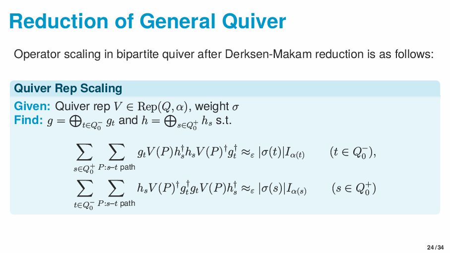
Derksen-Makam reduction is as follows: Quiver Rep Scaling Given: Quiver rep V ∈ Rep(Q, α), weight σ Find: g = t∈Q− 0 gt and h = s∈Q+ 0 hs s.t. s∈Q+ 0 P:s–t path gt V (P)h† s hs V (P)†g† t ≈ε |σ(t)|Iα(t) (t ∈ Q− 0 ), t∈Q− 0 P:s–t path hs V (P)†g† t gt V (P)h† s ≈ε |σ(s)|Iα(s) (s ∈ Q+ 0 ) 24 / 34
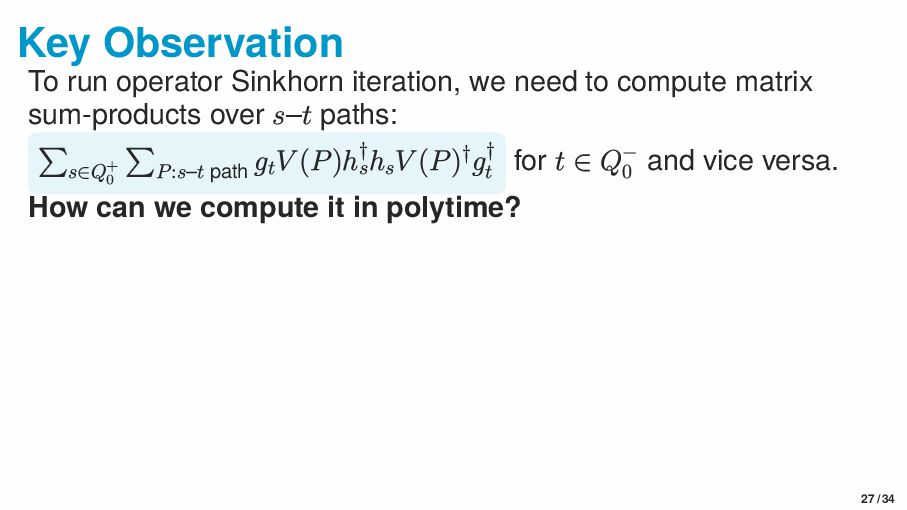
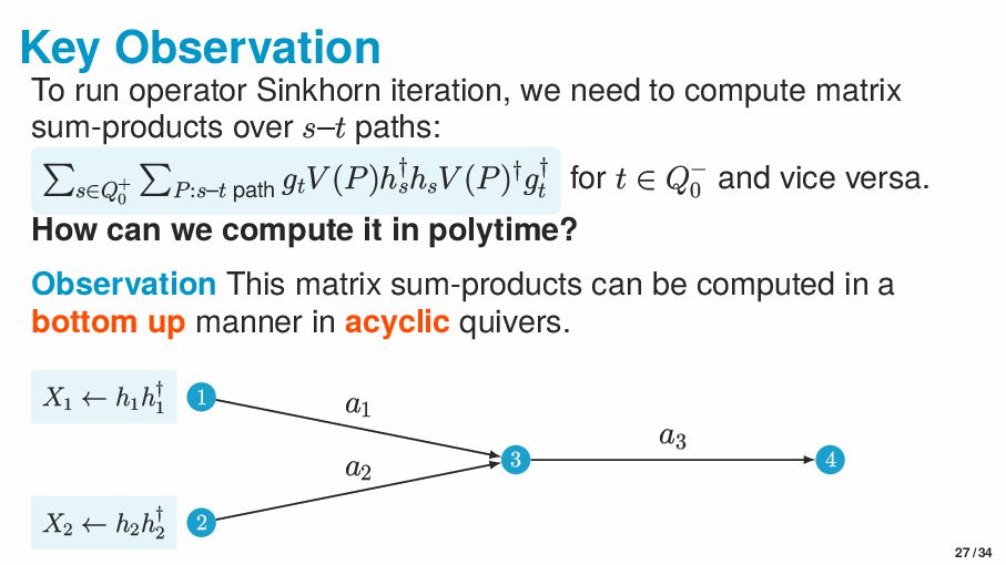
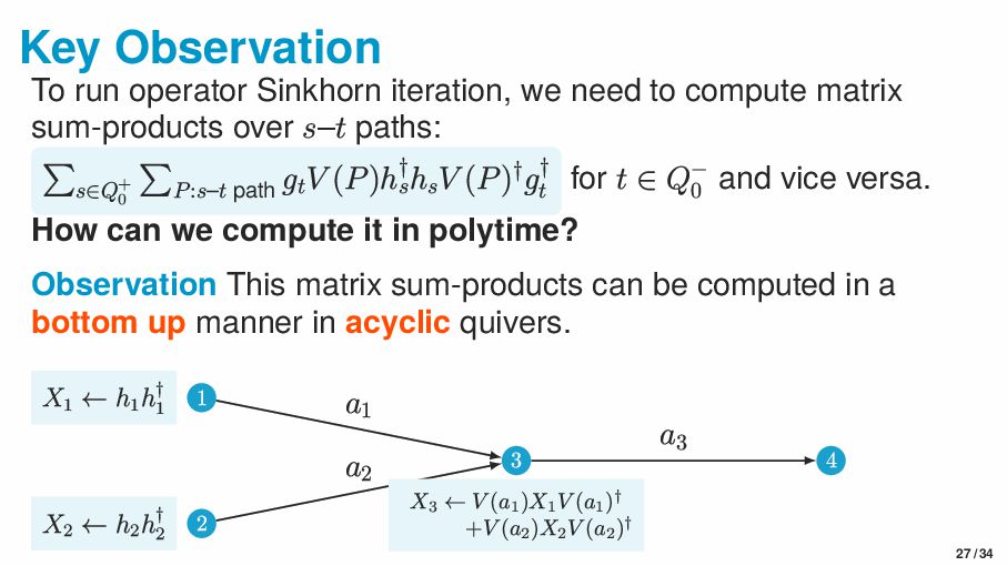
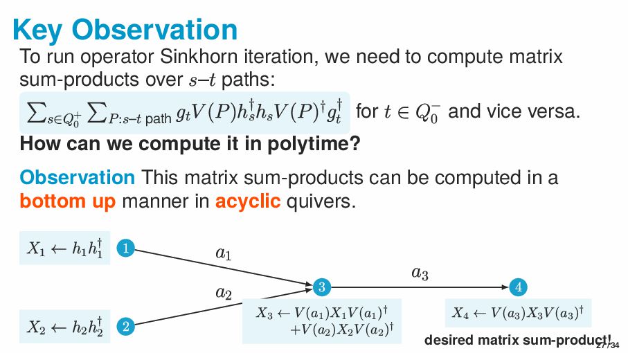
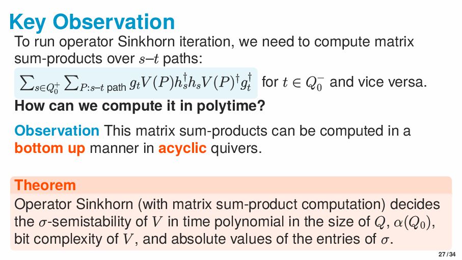
compute matrix sum-products over s–t paths: s∈Q+ 0 P:s–t path gt V (P)h† s hs V (P)†g† t for t ∈ Q− 0 and vice versa. How can we compute it in polytime? 27 / 34
compute matrix sum-products over s–t paths: s∈Q+ 0 P:s–t path gt V (P)h† s hs V (P)†g† t for t ∈ Q− 0 and vice versa. How can we compute it in polytime? Observation This matrix sum-products can be computed in a bottom up manner in acyclic quivers. 1 2 3 4 a1 a3 a2 X1 ← h1 h† 1 X2 ← h2 h† 2 X3 ← V (a1 )X1 V (a1 )† +V (a2 )X2 V (a2 )† X4 ← V (a3 )X3 V (a3 )† desired matrix sum-product! 27 / 34
compute matrix sum-products over s–t paths: s∈Q+ 0 P:s–t path gt V (P)h† s hs V (P)†g† t for t ∈ Q− 0 and vice versa. How can we compute it in polytime? Observation This matrix sum-products can be computed in a bottom up manner in acyclic quivers. 1 2 3 4 a1 a3 a2 X1 ← h1 h† 1 X2 ← h2 h† 2 X3 ← V (a1 )X1 V (a1 )† +V (a2 )X2 V (a2 )† X4 ← V (a3 )X3 V (a3 )† desired matrix sum-product! 27 / 34
compute matrix sum-products over s–t paths: s∈Q+ 0 P:s–t path gt V (P)h† s hs V (P)†g† t for t ∈ Q− 0 and vice versa. How can we compute it in polytime? Observation This matrix sum-products can be computed in a bottom up manner in acyclic quivers. 1 2 3 4 a1 a3 a2 X1 ← h1 h† 1 X2 ← h2 h† 2 X3 ← V (a1 )X1 V (a1 )† +V (a2 )X2 V (a2 )† X4 ← V (a3 )X3 V (a3 )† desired matrix sum-product! 27 / 34
compute matrix sum-products over s–t paths: s∈Q+ 0 P:s–t path gt V (P)h† s hs V (P)†g† t for t ∈ Q− 0 and vice versa. How can we compute it in polytime? Observation This matrix sum-products can be computed in a bottom up manner in acyclic quivers. Theorem Operator Sinkhorn (with matrix sum-product computation) decides the σ-semistability of V in time polynomial in the size of Q, α(Q0 ), bit complexity of V , and absolute values of the entries of σ. 27 / 34
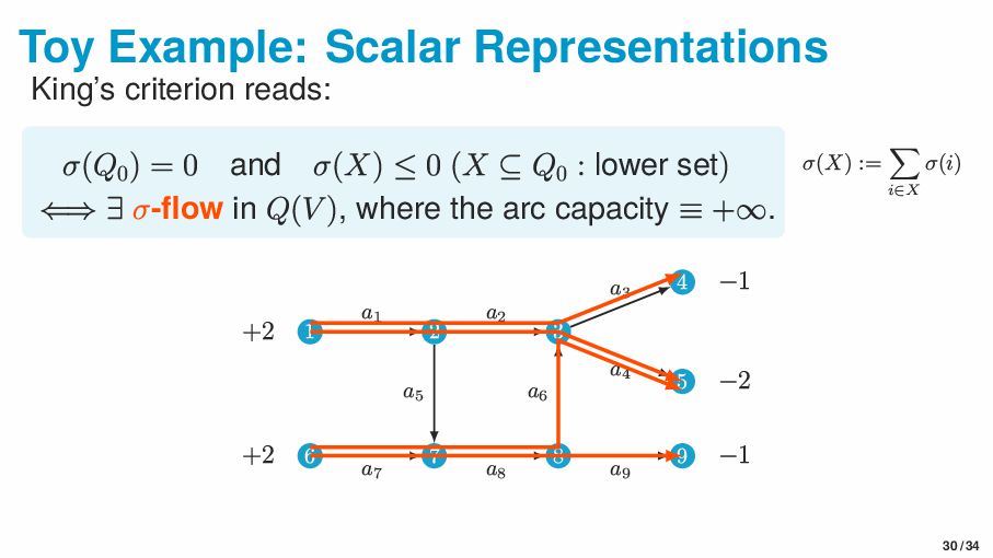
acyclic quiver is σ-semistable if and only if σ(dim V ) = 0 and σ(dim W) ≤ 0 (W ≤ V ) King’s cone For a rep V of an acyclic quiver, define King’s cone as a set of σ ∈ RQ0 s.t. σ(dim V ) = 0 and σ(dim W) ≤ 0 (W ≤ V ) This polyhedral cone has nice connections to network flow! 28 / 34
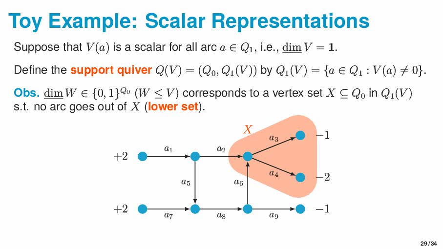
scalar for all arc a ∈ Q1 , i.e., dim V = 1. Define the support quiver Q(V ) = (Q0 , Q1 (V )) by Q1 (V ) = {a ∈ Q1 : V (a) ̸= 0}. Obs. dim W ∈ {0, 1}Q0 (W ≤ V ) corresponds to a vertex set X ⊆ Q0 in Q1 (V ) s.t. no arc goes out of X (lower set). X a1 a2 a3 a4 a7 a8 a9 a5 a6 +2 +2 −1 −2 −1 29 / 34
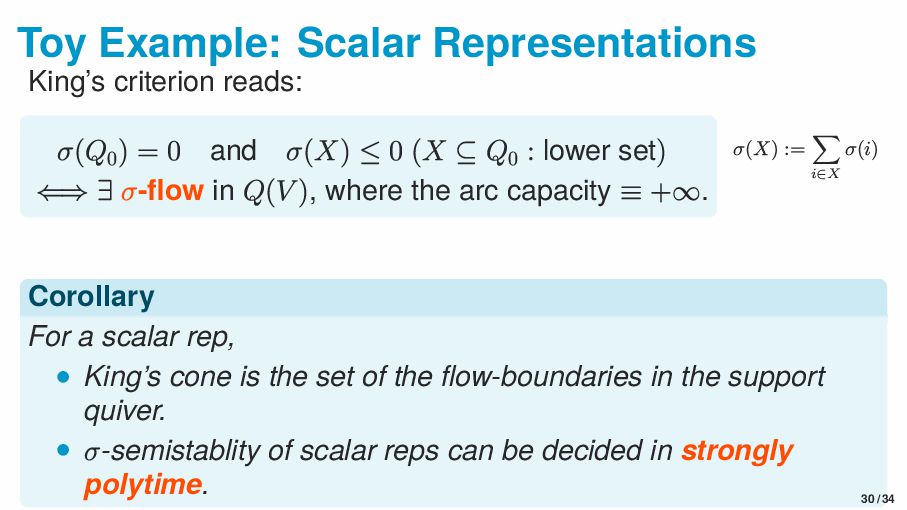
0 and σ(X) ≤ 0 (X ⊆ Q0 : lower set) ⇐⇒ ∃ σ-flow in Q(V ), where the arc capacity ≡ +∞. σ(X) := i∈X σ(i) Corollary For a scalar rep, • King’s cone is the set of the flow-boundaries in the support quiver. • σ-semistablity of scalar reps can be decided in strongly polytime. 30 / 34
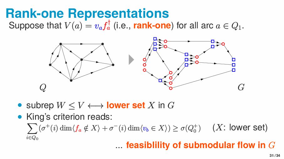
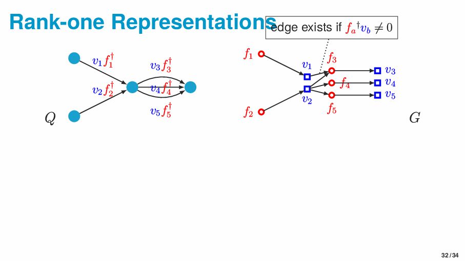
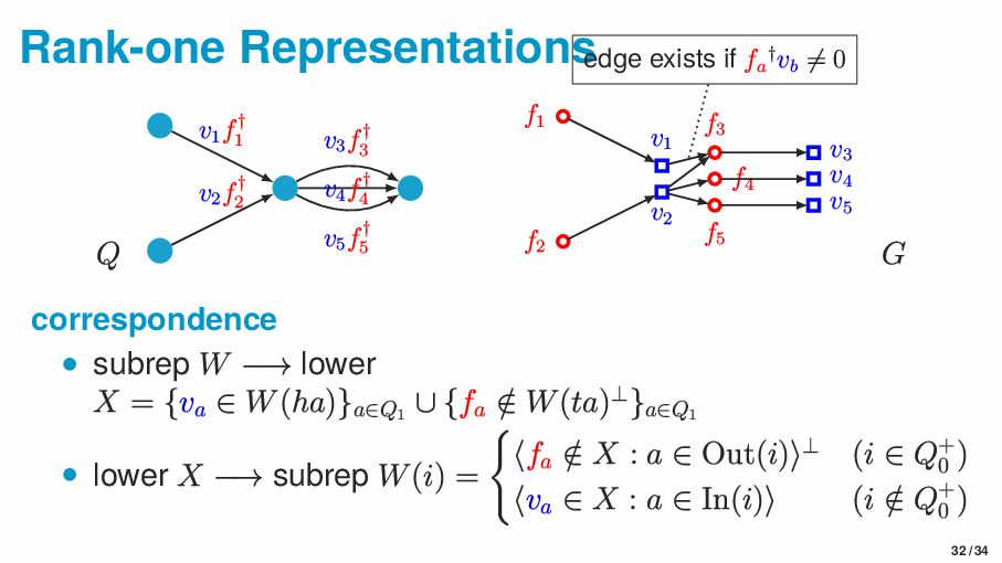
(i.e., rank-one) for all arc a ∈ Q1 . Q G • subrep W ≤ V ←→ lower set X in G • King’s criterion reads: i∈Q0 (σ+(i) dim⟨fa / ∈ X⟩ + σ−(i) dim⟨vb ∈ X⟩) ≥ σ(Q+ 0 ) (X: lower set) ... feasiblility of submodular flow in G 31 / 34
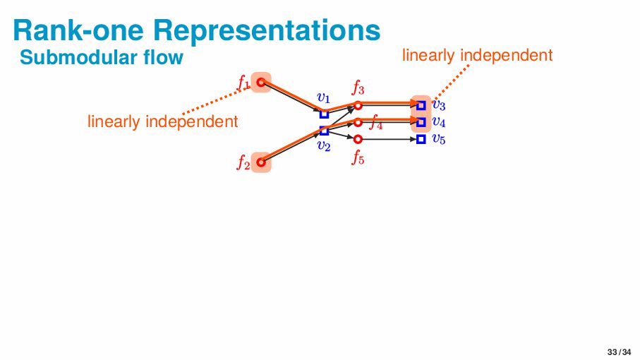
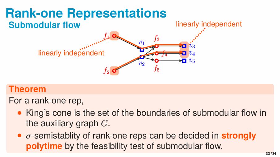
f5 v3 v4 v5 linearly independent linearly independent Theorem For a rank-one rep, • King’s cone is the set of the boundaries of submodular flow in the auxiliary graph G. • σ-semistablity of rank-one reps can be decided in strongly polytime by the feasibility test of submodular flow. 33 / 34
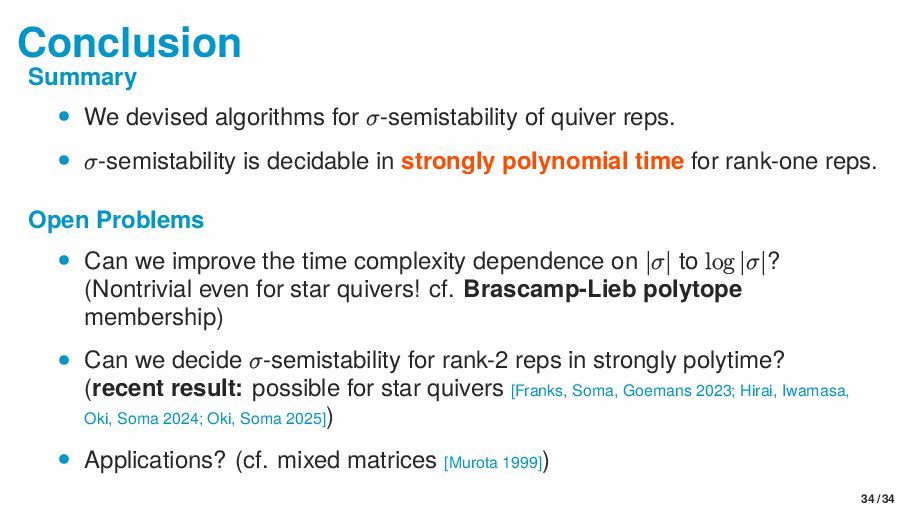
reps. • σ-semistability is decidable in strongly polynomial time for rank-one reps. Open Problems • Can we improve the time complexity dependence on |σ| to log |σ|? (Nontrivial even for star quivers! cf. Brascamp-Lieb polytope membership) • Can we decide σ-semistability for rank-2 reps in strongly polytime? (recent result: possible for star quivers [Franks, Soma, Goemans 2023; Hirai, Iwamasa, Oki, Soma 2024; Oki, Soma 2025]) • Applications? (cf. mixed matrices [Murota 1999]) 34 / 34
![King’s Criterion [King 1994] A characterization of σ-semistability by a](https://files.speakerdeck.com/presentations/957fac92013f44e580e19a832c04ec5f/slide_20.jpg)
![King’s Criterion [King 1994] A characterization of σ-semistability by a](https://files.speakerdeck.com/presentations/957fac92013f44e580e19a832c04ec5f/slide_21.jpg)
![King’s Criterion [King 1994] A characterization of σ-semistability by a](https://files.speakerdeck.com/presentations/957fac92013f44e580e19a832c04ec5f/slide_22.jpg)
![Reduction to Bipartite Quivers [Derksen, Makam 2017] Let • Q+](https://files.speakerdeck.com/presentations/957fac92013f44e580e19a832c04ec5f/slide_29.jpg)
![Reduction to Bipartite Quivers [Derksen, Makam 2017] Let • Q+](https://files.speakerdeck.com/presentations/957fac92013f44e580e19a832c04ec5f/slide_30.jpg)
![Reduction to Bipartite Quivers [Derksen, Makam 2017] Q+ 0 Q−](https://files.speakerdeck.com/presentations/957fac92013f44e580e19a832c04ec5f/slide_31.jpg)
![Reduction to Bipartite Quivers [Derksen, Makam 2017] Q+ 0 Q−](https://files.speakerdeck.com/presentations/957fac92013f44e580e19a832c04ec5f/slide_32.jpg)
![Operator Scaling with Specified Marginals [Franks 2018] Given: matrices A1](https://files.speakerdeck.com/presentations/957fac92013f44e580e19a832c04ec5f/slide_33.jpg)
![Operator Sinkhorn Iteration [Gurvits 2004; Franks 2018] Until convergence do:](https://files.speakerdeck.com/presentations/957fac92013f44e580e19a832c04ec5f/slide_34.jpg)
![Operator Sinkhorn Iteration [Gurvits 2004; Franks 2018] Until convergence do:](https://files.speakerdeck.com/presentations/957fac92013f44e580e19a832c04ec5f/slide_35.jpg)