Accelerating operator Sinkhorn iteration with overrelaxation

The 9th ISM-IIR-ZIB-NUS-NII-MODAL Workshop on Optimization

Transcript

1. Accelerating operator Sinkhorn iteration with overrelaxation Tasuku Soma (ISM / RIKEN AIP) André Uschmajew (University of Augsburg) 1 / 19
2. 1 Operator Scaling 2 Proposed Methods 3 Numerical Experiments 2 / 19
3. 1 Operator Scaling 2 Proposed Methods 3 Numerical Experiments 3 / 19
4. Operator Scaling [Gurvits 2004] Input: Matrices A1 , . . . , Ak ∈ Rm×n Output: Invertible matrices (L, R) ∈ GL(m) × GL(n) such that ˜ Ai := LAi R⊤ satisfy k i=1 ˜ Ai ˜ A⊤ i = 1 m Im , k i=1 ˜ A⊤ i ˜ Ai = 1 n In . • Generalization of matrix scaling [Sinkhorn 1964] (popular in ML to approx OT) • Edmonds’ problem [Gurvits 2004; Garg, Gurvits, Oliveira, Wigderson 2020] • Brascamp–Lieb inequality [Garg, Gurvits, Oliveira, Wigderson 2018] • Tyler’s M-estimator [Franks, Moitra 2020], covariance estimation for matrix normal distribution [Dutilleul 1999; Drton, Kuriki, Hoff 2021] 4 / 19
5. Operator Sinkhorn Iteration [Gurvits 2004] Generalization of Sinkhorn iteration for matrix scaling [Sinkhorn 1964] ˜ A(2t+1) i = L ˜ A(2t) i where L satisfies L k i=1 ˜ A(2t) i ˜ A(2t)⊤ i L⊤ = Im m ˜ A(2t+2) i = ˜ A(2t+1) i R⊤ where R satisfies R k i=1 ˜ A(2t+1)⊤ i ˜ A(2t+1) i R⊤ = In n L, R can be easily computed by Cholesky or matrix square roots 5 / 19
6. Operator Sinkhorn Iteration [Gurvits 2004] Generalization of Sinkhorn iteration for matrix scaling [Sinkhorn 1964] ˜ A(2t+1) i = L ˜ A(2t) i where L satisfies L k i=1 ˜ A(2t) i ˜ A(2t)⊤ i L⊤ = Im m ˜ A(2t+2) i = ˜ A(2t+1) i R⊤ where R satisfies R k i=1 ˜ A(2t+1)⊤ i ˜ A(2t+1) i R⊤ = In n L, R can be easily computed by Cholesky or matrix square roots Theorem (Gurvits (2004)) If a solution to operator scaling exists, the operator Sinkhorn iteration ( ˜ A(t) i ) converges to a solution. 5 / 19
7. Application: Covariance Estimation [Drton, Kuriki, Hoff 2021] G: d × d matrix with i.i.d. standard normal entries L: d × d1 matrix, R: d × d2 matrix The distribution of L⊤GR is called the matrix normal distribution. Its covariance matrix is Σ2 ⊗ Σ1 , where Σ1 := R⊤R, Σ2 := L⊤L. L⊤ G ∼ N(0, 1) R 6 / 19
8. Application: Covariance Estimation [Drton, Kuriki, Hoff 2021] G: d × d matrix with i.i.d. standard normal entries L: d × d1 matrix, R: d × d2 matrix The distribution of L⊤GR is called the matrix normal distribution. Its covariance matrix is Σ2 ⊗ Σ1 , where Σ1 := R⊤R, Σ2 := L⊤L. L⊤ G ∼ N(0, 1) R Given data A1 , . . . , Am , the log-likelihood function is ℓ(Σ1 , Σ2 ) = − 1 2 tr m i=1 Σ−1 2 A⊤ i Σ−1 1 Ai − d2 2 log det Σ1 − d1 2 log det Σ2 + const. • With the change of variables (X, Y ) ← (Σ−1 1 , Σ−1 2 ), finding a stationary point of log-likelihood ℓ is equivalent to operator scaling. • Operator Sinkhorn iteration was previously known as the flip-flop algorithm [Dutilleul 1999]. 6 / 19
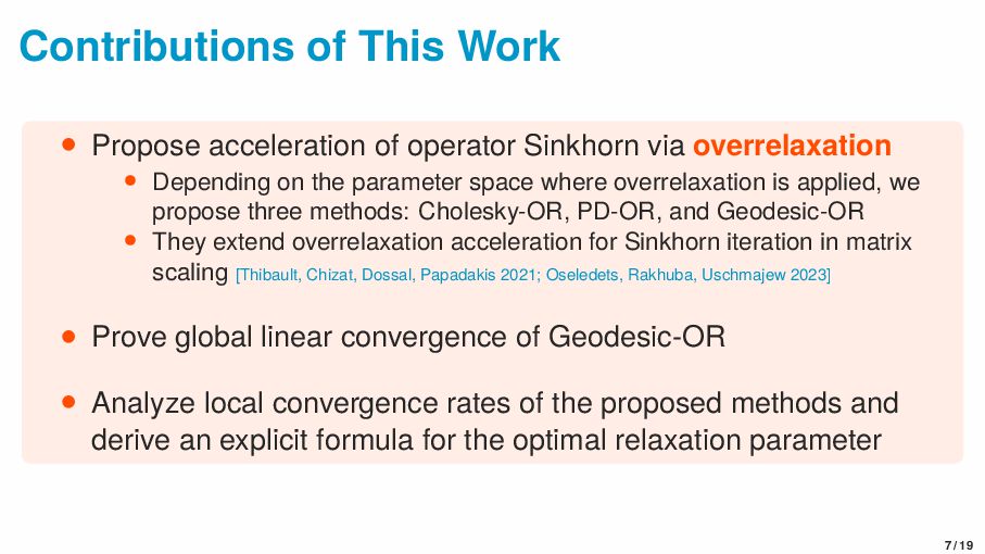
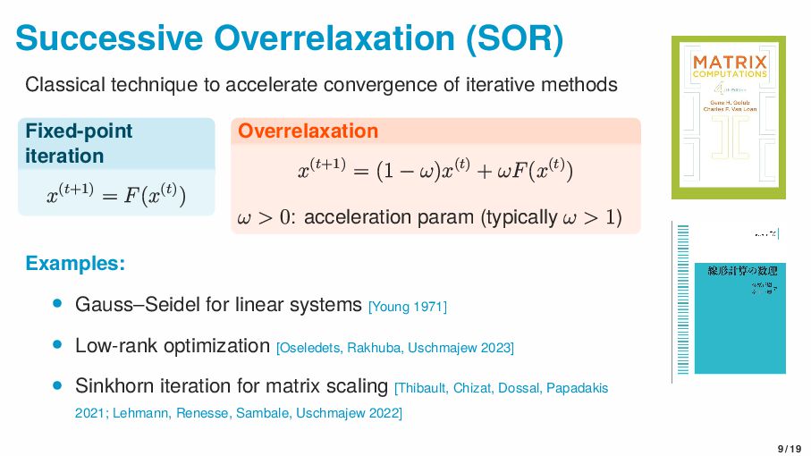
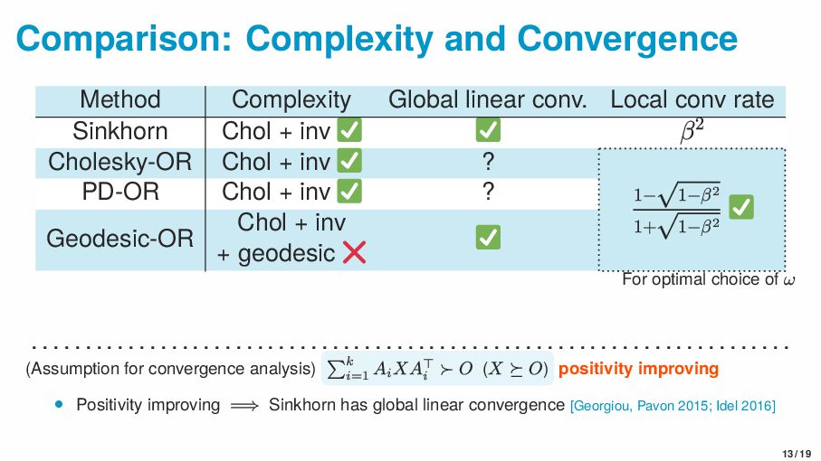
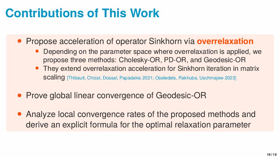
9. Contributions of This Work • Propose acceleration of operator Sinkhorn via overrelaxation • Depending on the parameter space where overrelaxation is applied, we propose three methods: Cholesky-OR, PD-OR, and Geodesic-OR • They extend overrelaxation acceleration for Sinkhorn iteration in matrix scaling [Thibault, Chizat, Dossal, Papadakis 2021; Oseledets, Rakhuba, Uschmajew 2023] • Prove global linear convergence of Geodesic-OR • Analyze local convergence rates of the proposed methods and derive an explicit formula for the optimal relaxation parameter 7 / 19
10. 1 Operator Scaling 2 Proposed Methods 3 Numerical Experiments 8 / 19
11. Successive Overrelaxation (SOR) Classical technique to accelerate convergence of iterative methods Fixed-point iteration x(t+1) = F(x(t)) Overrelaxation x(t+1) = (1 − ω)x(t) + ωF(x(t)) ω > 0: acceleration param (typically ω > 1) Examples: • Gauss–Seidel for linear systems [Young 1971] • Low-rank optimization [Oseledets, Rakhuba, Uschmajew 2023] • Sinkhorn iteration for matrix scaling [Thibault, Chizat, Dossal, Papadakis 2021; Lehmann, Renesse, Sambale, Uschmajew 2022] 9 / 19
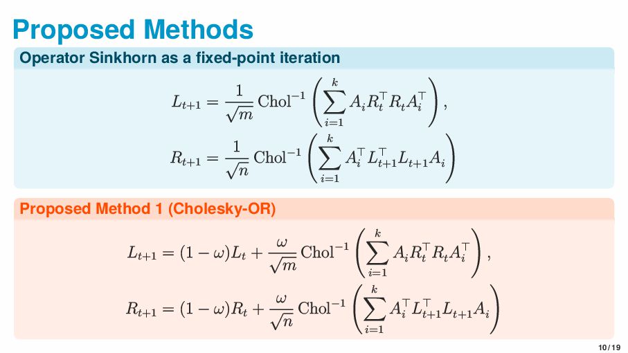
12. Proposed Methods Operator Sinkhorn as a fixed-point iteration Lt+1 = 1 √ m Chol−1 k i=1 Ai R⊤ t Rt A⊤ i , Rt+1 = 1 √ n Chol−1 k i=1 A⊤ i L⊤ t+1 Lt+1 Ai Proposed Method 1 (Cholesky-OR) Lt+1 = (1 − ω)Lt + ω √ m Chol−1 k i=1 Ai R⊤ t Rt A⊤ i , Rt+1 = (1 − ω)Rt + ω √ n Chol−1 k i=1 A⊤ i L⊤ t+1 Lt+1 Ai 10 / 19
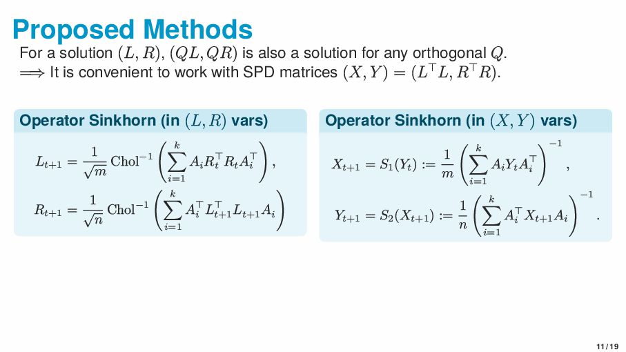
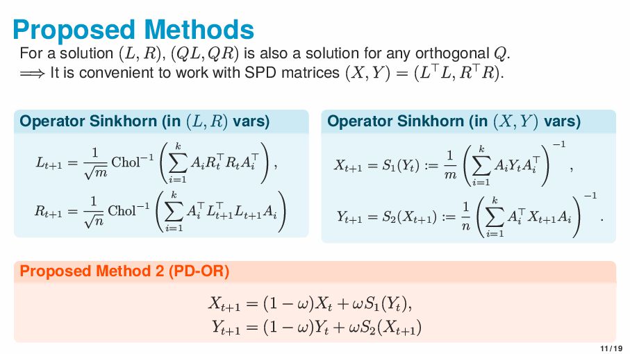
13. Proposed Methods For a solution (L, R), (QL, QR) is also a solution for any orthogonal Q. =⇒ It is convenient to work with SPD matrices (X, Y ) = (L⊤L, R⊤R). Operator Sinkhorn (in (L, R) vars) Lt+1 = 1 √ m Chol−1 k i=1 Ai R⊤ t Rt A⊤ i , Rt+1 = 1 √ n Chol−1 k i=1 A⊤ i L⊤ t+1 Lt+1 Ai Operator Sinkhorn (in (X, Y ) vars) Xt+1 = S1 (Yt ) := 1 m k i=1 Ai Yt A⊤ i −1 , Yt+1 = S2 (Xt+1 ) := 1 n k i=1 A⊤ i Xt+1 Ai −1 . 11 / 19
14. Proposed Methods For a solution (L, R), (QL, QR) is also a solution for any orthogonal Q. =⇒ It is convenient to work with SPD matrices (X, Y ) = (L⊤L, R⊤R). Operator Sinkhorn (in (L, R) vars) Lt+1 = 1 √ m Chol−1 k i=1 Ai R⊤ t Rt A⊤ i , Rt+1 = 1 √ n Chol−1 k i=1 A⊤ i L⊤ t+1 Lt+1 Ai Operator Sinkhorn (in (X, Y ) vars) Xt+1 = S1 (Yt ) := 1 m k i=1 Ai Yt A⊤ i −1 , Yt+1 = S2 (Xt+1 ) := 1 n k i=1 A⊤ i Xt+1 Ai −1 . Proposed Method 2 (PD-OR) Xt+1 = (1 − ω)Xt + ωS1 (Yt ), Yt+1 = (1 − ω)Yt + ωS2 (Xt+1 ) 11 / 19
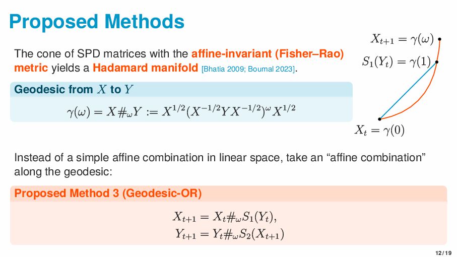
15. Proposed Methods The cone of SPD matrices with the affine-invariant (Fisher–Rao) metric yields a Hadamard manifold [Bhatia 2009; Boumal 2023]. Geodesic from X to Y γ(ω) = X#ω Y := X1/2(X−1/2Y X−1/2)ωX1/2 Xt = γ(0) S1 (Yt ) = γ(1) Xt+1 = γ(ω) Instead of a simple affine combination in linear space, take an “affine combination” along the geodesic: Proposed Method 3 (Geodesic-OR) Xt+1 = Xt #ω S1 (Yt ), Yt+1 = Yt #ω S2 (Xt+1 ) 12 / 19
16. Comparison: Complexity and Convergence Method Complexity Global linear conv. Local conv rate Sinkhorn Chol + inv β2 Cholesky-OR Chol + inv ? PD-OR Chol + inv ? Geodesic-OR 1− √ 1−β2 1+ √ 1−β2 Chol + inv + geodesic For optimal choice of ω . . . . . . . . . . . . . . . . . . . . . . . . . . . . . . . . . . . . . . . . . . . . . . . . . . . . . . . . . . . . . . . . . . . . . . . (Assumption for convergence analysis) k i=1 Ai XA⊤ i ≻ O (X ⪰ O) positivity improving • Positivity improving =⇒ Sinkhorn has global linear convergence [Georgiou, Pavon 2015; Idel 2016] 13 / 19
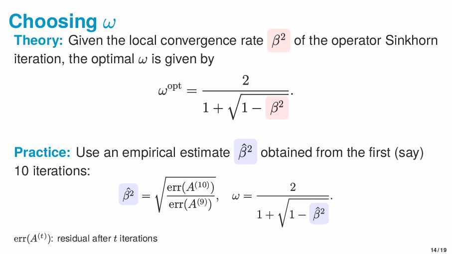
17. Choosing ω Theory: Given the local convergence rate β2 of the operator Sinkhorn iteration, the optimal ω is given by ωopt = 2 1 + 1 − β2 . Practice: Use an empirical estimate ˆ β2 obtained from the first (say) 10 iterations: ˆ β2 = err(A(10)) err(A(9)) , ω = 2 1 + 1 − ˆ β2 . err(A(t)): residual after t iterations 14 / 19
18. 1 Operator Scaling 2 Proposed Methods 3 Numerical Experiments 15 / 19
19. Numerical Experiments We test on the following instance of operator scaling. Frame Scaling [Holmes, Paulsen 2004; Barthe 1998; Tyler 1987] Input vectors x1 , . . . , xk ∈ Rn Output Invertible P ∈ GLn (R), scalars α1 , . . . , αk ≥ 0 s.t. ˜ xi = αi Pxi satisfy ∥˜ xi ∥2 2 = n k (i = 1, . . . , k), k i=1 ˜ xi ˜ x⊤ i = In . (Perseval frame) Experimental Setup • n = 50, k = 55 • xi ∼ N(0, In ) • Error metric: gradnorm := i (∥˜ xi ∥2 2 − n/k)2 + i ˜ xi ˜ x⊤ i − In 2 F 16 / 19
20. Results (Iterations vs Error) 0 25 50 75 100 125 150 175 200 iteration 10 14 10 12 10 10 10 8 10 6 10 4 10 2 grad norm Cholesky-OR: omega=1.59250 Geodesic-OR: omega=1.59250 PD-OR: omega=1.59250 OSI Proposed methods are about 4x faster than Sinkhorn. 17 / 19
21. Results (Time vs Error) 0.0 0.5 1.0 1.5 2.0 2.5 3.0 3.5 4.0 time [s] 10 14 10 12 10 10 10 8 10 6 10 4 10 2 grad norm Cholesky-OR: omega=1.59250 Geodesic-OR: omega=1.59250 PD-OR: omega=1.59250 OSI Proposed methods are about 3x faster than Sinkhorn. Geodesic-OR is slightly slower. 18 / 19
22. Contributions of This Work • Propose acceleration of operator Sinkhorn via overrelaxation • Depending on the parameter space where overrelaxation is applied, we propose three methods: Cholesky-OR, PD-OR, and Geodesic-OR • They extend overrelaxation acceleration for Sinkhorn iteration in matrix scaling [Thibault, Chizat, Dossal, Papadakis 2021; Oseledets, Rakhuba, Uschmajew 2023] • Prove global linear convergence of Geodesic-OR • Analyze local convergence rates of the proposed methods and derive an explicit formula for the optimal relaxation parameter 19 / 19
23. 4 Convergence Analysis 1 / 4
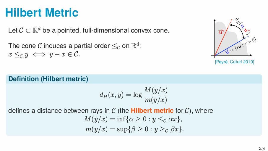
24. Hilbert Metric Let C ⊂ Rd be a pointed, full-dimensional convex cone. The cone C induces a partial order ≤C on Rd: x ≤C y ⇐⇒ y − x ∈ C. 68 ! u 0 ! u = {ru ; r > 0} dH (u,u 0 ) Figure 4.7: Left: the Hilber vizualization of the contracti It can be shown to be means that ∃r > 0, u naming “projective”). dH(u, u ) = 0 if and on distance on bounded o is a complete metric s the Hilbert metric on norm between vectors [Peyré, Cuturi 2019] Definition (Hilbert metric) dH (x, y) = log M(y/x) m(y/x) defines a distance between rays in C (the Hilbert metric for C), where M(y/x) = inf{α ≥ 0 : y ≤C αx}, m(y/x) = sup{β ≥ 0 : y ≥C βx}. 2 / 4
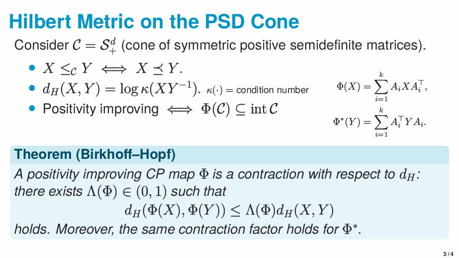
25. Hilbert Metric on the PSD Cone Consider C = Sd + (cone of symmetric positive semidefinite matrices). • X ≤C Y ⇐⇒ X ⪯ Y . • dH (X, Y ) = log κ(XY −1). κ(·) = condition number • Positivity improving ⇐⇒ Φ(C) ⊆ int C Φ(X) = k i=1 Ai XA⊤ i , Φ∗(Y ) = k i=1 A⊤ i Y Ai . Theorem (Birkhoff–Hopf) A positivity improving CP map Φ is a contraction with respect to dH : there exists Λ(Φ) ∈ (0, 1) such that dH (Φ(X), Φ(Y )) ≤ Λ(Φ)dH (X, Y ) holds. Moreover, the same contraction factor holds for Φ∗. 3 / 4
26. Global Convergence Lemma dH (X#ω Y, Z) ≤ |1 − ω| dH (X, Z) + ω dH (Y, Z) (ω ≥ 0) Note: In particular, for ω ∈ [0, 1], this shows (Sd ++ / ∼, dH ) is a Busemann space [Gunawardena, Walsh 2003]. Convergence Analysis dH (X(t), X∗) = dH (X(t−1)#ω S1 (Y (t−1)), X∗) ≤ |1 − ω|dH (X(t−1), X∗) + ωdH (S1 (Y (t−1)), S1 (Y ∗)) ≤ |1 − ω|dH (X(t−1), X∗) + ωΛdH (Y (t−1), Y ∗). Hence, dH (X(t), X∗) dH (Y (t), Y ∗) ≤ |1 − ω| ωΛ ωΛ|1 − ω| |1 − ω| + (ωΛ)2 dH (X(t−1), X∗) dH (Y (t−1), Y ∗) The spectral radius of this matrix is less than 1 if 0 < ω < 2/(1 + Λ), so the method converges globally. 4 / 4