Data Mining with the Heritage Health Prize

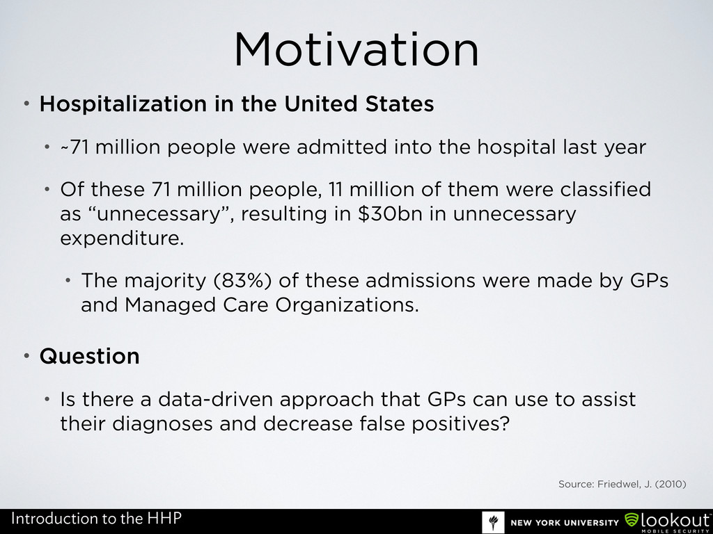
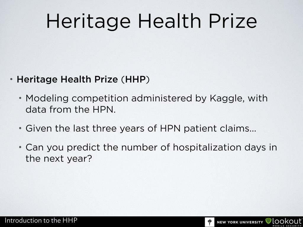
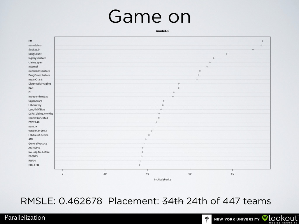
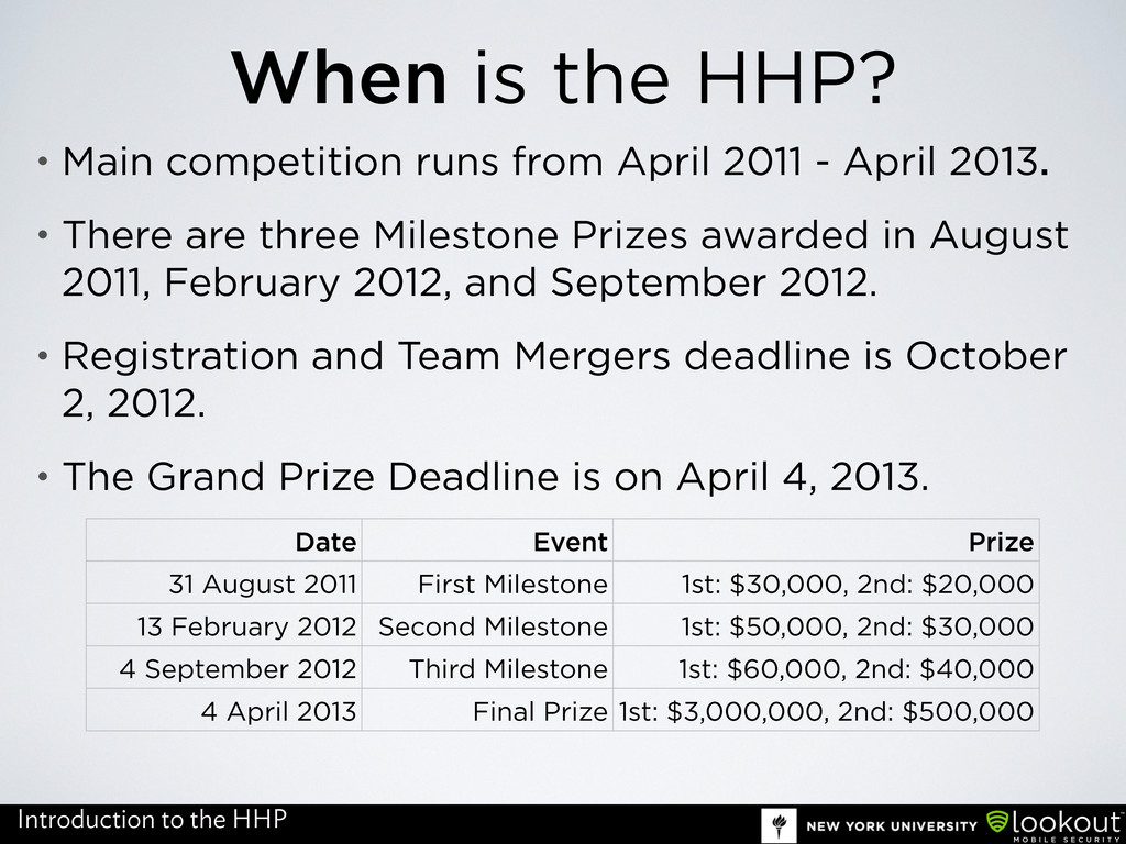
This is a slide deck for a lightning talk I gave at the Bay Area R Users Group meetup on 13 December 2011. It covers a brief run-through of the work I did on the Heritage Health prize up to the first checkpoint Prize (August 2011).

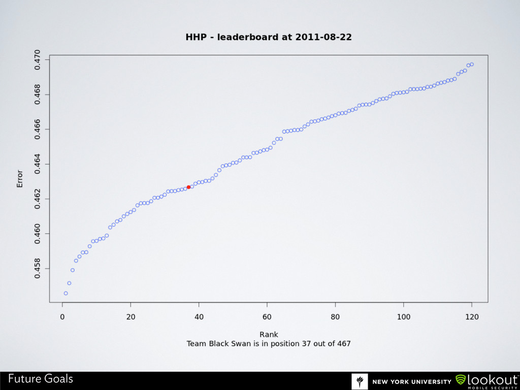
PS The rankings on the slide deck are sadly no longer accurate! I'm like 421349876th place now. Oh well.

Transcript

1. The Heritage Health Prize Thomson Nguyen 13 December 2011 Modeling Healthcare in Ten Minutes email thomson@cantab.net twitter @itsthomson Data Mining with R: Lightning Talks
2. Hi, I’m Thomson. Currently: Data scientist at Lookout Mobile Security, visiting scholar at NYU Courant. I enjoy: Rowing, road cycling, SC2, finding good rueben sandwich places. This presentation: Covers my work on the HHP as a Research Visitor at NYU Courant with Prof. Bud Mishra. About Me
3. Agenda • Introduction to the Heritage Health Prize • The Datasets • Preliminary Models • Random Decision Trees • Parallelization • Summary
4. Introduction to the HHP The Datasets Preliminary Models Random Decision Trees Parallelization
5. Motivation • Hospitalization in the United States • ~71 million people were admitted into the hospital last year • Of these 71 million people, 11 million of them were classified as “unnecessary”, resulting in $30bn in unnecessary expenditure. • The majority (83%) of these admissions were made by GPs and Managed Care Organizations. • Question • Is there a data-driven approach that GPs can use to assist their diagnoses and decrease false positives? Source: Friedwel, J. (2010) Introduction to the HHP
6. Heritage Health Prize • Heritage Health Prize (HHP) • Modeling competition administered by Kaggle, with data from the HPN. • Given the last three years of HPN patient claims... • Can you predict the number of hospitalization days in the next year? Introduction to the HHP
7. Introduction to the HHP The Datasets Preliminary Models Random Decision Trees Parallelization Future Goals
8. What’s in the data? The Datasets Members Table (113000 x 3) Claims Table (Randomized claims for Y1, Y2, Y3, 2668990 x 14) Labs Table (361484 x 4) DaysInHospital Tables (Y2/Y3) > head(members) MemberID AgeAtFirstClaim Sex 1 14723353 70-79 M 2 75706636 70-79 M 3 17320609 70-79 M 4 69690888 40-49 M 5 33004608 0-9 M 6 63690883 40-49 F > head(claims) MemberID ProviderID Vendor PCP Year Specialty PlaceSvc PayDelay DSFS PCG CharlsonIndex ProcedureGroup SupLOS 1 42286978 8013252 172193 37796 Y1 Surgery Office 28 8- 9 months NEUMENT 0 MED 0 2 97903248 3316066 726296 5300 Y3 Internal Office 50 8- 9 months NEUMENT 0 MED 1 3 2759427 2997752 140343 91972 Y3 Internal Office 14 0- 1 month METAB3 0 EM 1 4 73570559 7053364 240043 70119 Y3 Laboratory Independent Lab 24 0- 1 month METAB3 0 SCS 0 5 11837054 7557061 496247 68968 Y2 Surgery Outpatient Hospital 27 4- 5 months FXDISLC 1-2 EM 1 6 45844561 1963488 4042 55823 Y3 Pediatrics Office 25 3- 4 months NEUMENT 0 EM 0 > head(drug.count) MemberID Year DSFS DrugCount 1 48925661 Y2 9-10 months 7+ 2 90764620 Y3 8- 9 months 3 3 61221204 Y1 2- 3 months 1 4 63628544 Y3 1- 2 months 1 5 46949606 Y2 10-11 months 3 6 72110751 Y2 9-10 months 1 Rx Table (Y1/Y2/Y3, 818241 x 4) > head(lab.count) MemberID Year DSFS LabCount 1 69258001 Y3 2- 3 months 1 2 10143167 Y1 0- 1 month 2 3 1054357 Y1 0- 1 month 6 4 56583841 Y3 6- 7 months 4 5 70967047 Y2 0- 1 month 2 6 88850854 Y2 3- 4 months 5 > head(hospital.y2) MemberID ClaimsTruncated DaysInHospital 1 24027423 0 0 2 98324177 0 0 3 33899367 1 1 4 5481382 0 1 5 69908334 0 0 6 29951458 0 0 Right censored at 15 days! The Datasets
9. Bringing it Together The Datasets • Split claims by year, use only claims that are attached to a member with a hospitalization record: getCleanClaims <- function(x="Y1", y=hospital.y2){ sand <- claims[claims$Year==x,] all.in <- sand$MemberID %in% y$MemberID sand <- sand[all.in,] } > clean.1 <- getCleanClaims("Y1", hospital.y2) > clean.2 <- getCleanClaims("Y2", hospital.y3) > clean.3 <- getCleanClaims("Y3", hospital.y4) • Create tables of `counts’ for each factor and merge it with Members.csv: makeTab <- function(x,y) { temp <- table(x,y) class(temp) <- "matrix" temp <- as.data.frame(temp, stringsAsFactors = FALSE) temp <- cbind(row.names(temp),temp) temp[,1] <- as.numeric(as.character(temp[,1])) colnames(temp) <- c("MemberID",colnames(temp)[-1]) temp } > head(makeTab(clean.1$MemberID, clean.1$PlaceSvc)) MemberID Ambulance Home Independent Lab Inpatient Hospital Office 10000665 0 2 0 1 0 10001082 0 0 2 0 0 10001258 3 1 0 2 2 10001471 0 0 4 0 8 10001818 1 0 0 0 0 10002388 0 0 3 13 7 • Do this for all factors: 12 specialties, 8 places, 45 PCGs, 17 procedures, 5 Charlson indices, 1359 PCPs, 14699 ProviderIDs, and 6387 Vendors. The Datasets
10. Transform all of the things The Datasets • We now have three files (call them right files) with one unique member ID on each row and lots of columns: > dim(right.a) [1] 76038 22443 > dim(right.b) [1] 71435 22443 > dim(right.c) [1] 70942 22443 • Very sparse matrix! What does the data look like? > summary(right.a$Other.x) Min. 1st Qu. Median Mean 3rd Qu. Max. 0.00000 0.00000 0.00000 0.05086 0.00000 32.00000 That looks pretty skewed. What if we took the log(1+x) transform? > right.a$Other.x <- log1p(right.a$Other.x) > summary(right.a$Other.x) Min. 1st Qu. Median Mean 3rd Qu. Max. 0.00000 0.00000 0.00000 0.01878 0.00000 3.43200 It looks better? What did we just do? The Datasets
11. The Datasets
12. Introduction to the HHP The Datasets Preliminary Models Random Decision Trees Parallelization Future Goals
13. Model Evaluation • Entries will be judged by comparing • the predicted number of days a member will spend in the hospital reflected in the entry, • with the actual number of days a member spent in the hospital in DaysInHospital_Y4 (not given to competitors). • Prediction accuracy will be evaluated based on the following metric: This is the root mean squared log error (RMSLE) of an outcome. ￿ = ￿ ￿ ￿ ￿ 1 n n ￿ i [log(pi + 1) − log(ai + 1)]2 Preliminary Models
14. First Model Random Decision Trees
15. First Model Yi = β0 + β1φ1(Xi1) + · · · + βpφp(Xip) + ￿i • Recall a Linear Model: • Let’s create a simple linear regression of Age, and number of claims: > model.1 <- lm(log(DaysInHospital) ~ AgeAtFirstClaim + num.claims, data=training) > model.1 Call: lm(formula = log(DaysInHospital ~ AgeAtFirstClaim + num.claims) Coefficients: (Intercept) AgeAtFirstClaim num.claims -0.03551 0.07836 0.07504 > prediction <- predict(model, testing) > prediction <- expm1(prediction) > summary(prediction) Min. 1st Qu. Median Mean 3rd Qu. Max. 0.01664 0.10240 0.18400 0.20080 0.28700 0.51810 • RMSLE: 0.478246 (+.0918) , Placement: 82nd of 255 teams Preliminary Models
16. `Kitchen Sink’ Model • Let’s now add counts for all Condition Groups, Procedures, Place of care, and Charlson Comorbidity score: > model.1 <- lm(training[,2:105], log(training$DaysInHospital)) > prediction <- predict(model, testing) > prediction <- expm1(prediction) > summary(prediction) # Kitchen Sink model Min. 1st Qu. Median Mean 3rd Qu. Max. 0.00134 0.11240 0.19463 0.21892 0.28700 2.42792 > summary(prediction.old) # Three-variable model Min. 1st Qu. Median Mean 3rd Qu. Max. 0.01664 0.10240 0.18400 0.20080 0.28700 0.51810 • RMSLE: 0.463167 (+.0034) , Placement: 82nd 45th of 398 teams Preliminary Models
17. Preventing overfitting • Recursive Feature Selection • Train model with all predictors • Calculate model performance • Calculate variable importance/rankings For (S in seq(1, numPred, by = 1)) do Keep the S most important variables Train the model using these variables Calculate model performance Recalculate variable importance/rankings end • Calculate the model performance over all subsets S • Determine the final ranks of each predictor • Return list of predictors based on the optimal S value. Preliminary Models
18. Cross−validation scores with feature selection Number of variables in model RMSLE 0.44540 0.44545 0.44550 0.44555 0.44560 100 150 200 250 • • • • • • • • • • • • • • • • • • • • • • • • • • • • • • • • • • • • • • Optimized Kitchen Sink • RMSLE: 0.463002 (+.0021) • Placement: 45th 35th of 410 teams • Ran recursive feature selection on entire training set of 22443 predictors • Converged on 190 strongest predictors in linear model Preliminary Models
19. Introduction to the HHP The Datasets Preliminary Models Random Decision Trees Parallelisation Future Goals
20. Introduction to Decision Trees • Simple Decision Tree on Sex, PRGNCY, and CANCER1 • To create a tree, you take your training set and recursively partition subsets of predictors until splitting no longer adds value to the predictions. • Excellent for discrete data, but still prone to overfitting. Random Decision Trees
21. Random Decision Trees • Ensemble regressor that consists of many trees (in our case, ~500k) that are calculated on random subsets of the data, using random subsets of predictors for each tree split. • Each tree is fully grown (i.e. like computing a recursive partitioning 500k times) • To make a prediction, each test case is pushed down every tree and an average is taken for all trees. Random Decision Trees
22. > model.1 <- randomForest(x=model.training, y=model.training.response, ntree = 500000, nodesize=50, mtry=3,keep.forest=TRUE) RMSLE: 0.462973 Placement: 35th 34th of 427 teams Random Decision Trees
23. Just one problem... • Growing 500,000 trees with the competition data on a single Intel i7 desktop takes about seven hours. • Tuning and hill-climbing is infeasible. • We’re going to need to run this on multiple cores. > a <- Sys.time() > model.1 <- randomForest(x=model.training, y=model.training.response, ntree = 500000, nodesize=50, mtry=3,keep.forest=TRUE) > b <- Sys.time() > b - a Time difference of 7.336037 hours Random Decision Trees
24. Introduction to the HHP The Datasets Preliminary Models Random Decision Trees Parallelization Future Goals
25. Using foreach • foreach forks R as many times as you have cores (256). • With respect to randomForest, each core runs 2000 trees, • and then combines them into a ~500k forest when execution is finished. > a <- Sys.time() > registerDoMC(256) > mcoptions <- list(preschedule = FALSE, set.seed = FALSE) > model.1 <- foreach(ntree = rep(2000,256), .combine = combine, .packages = "randomForest") > %dopar% + randomForest(x=model.training, y=model.training.response, + ntree = ntree, nodesize=50, mtry=3, + .options.multicore=mcoptions,keep.forest=TRUE) > b <- Sys.time() Time difference of 3.19432 minutes Parallelization
26. Recursive Feature Selection, with mcapply • foreach forks R as many times as you have cores (256). • Same process as linear RFS, excepts runs a 500k randomForest for each subset of predictors. • Runs in total, about 10,000 500k randomForests. > control.rfe.rf <- rfeControl(functions = hhp.functions, rerank = TRUE, workers = 256, method = "repeatedcv", number = 25, returnResamp = "final", computeFunction = mclapply, computeArgs=list(mc.preschedule = FALSE, mc.set.seed = FALSE) ) > sizes <- seq(200, 24442 ,by=100) > model.1 <- rfe(model.training, model.training.response, sizes, metric = "HHP", maximize = FALSE, rfeControl = control.rfe.lm) Parallelization
27. Game on RMSLE: 0.462678 Placement: 34th 24th of 447 teams Parallelization
28. Introduction to the HHP The Datasets Preliminary Models Random Decision Trees Parallelisation Summary
29. Summary • Simple, robust models are easy and will get you places • Three variables put us in the top 40% • Visualizing data is always the first step • Anscombe’s Quartet • 80% of my time was spent cleaning the data • Better data will always beat better models Summary
30. Acknowledgments • Bud Mishra, for advising me on model selection and overall approaches to the HHP. • Fabian Menges and Giuseppe Narsizi for maintaining Courant Simulation Cluster. • NYU High Performance Computing Cluster for auxiliary simulations. • Nvidia for the Tesla GPUs and CUDA support. • Funding was provided by NYU Courant and NYU Langone Medical Center. Future Goals
31. Questions? End
32. Appendix
33. Looking at Claims.csv Claims Table (Randomized claims for Y1, Y2, Y3, 2668990 x 14) > head(claims) MemberID ProviderID Vendor PCP Year Specialty PlaceSvc PayDelay DSFS PCG CharlsonIndex ProcedureGroup SupLOS 1 42286978 8013252 172193 37796 Y1 Surgery Office 28 8- 9 months NEUMENT 0 MED 0 2 97903248 3316066 726296 5300 Y3 Internal Office 50 8- 9 months NEUMENT 0 MED 1 3 2759427 2997752 140343 91972 Y3 Internal Office 14 0- 1 month METAB3 0 EM 1 4 73570559 7053364 240043 70119 Y3 Laboratory Independent Lab 24 0- 1 month METAB3 0 SCS 0 5 11837054 7557061 496247 68968 Y2 Surgery Outpatient Hospital 27 4- 5 months FXDISLC 1-2 EM 1 6 45844561 1963488 4042 55823 Y3 Pediatrics Office 25 3- 4 months NEUMENT 0 EM 0 > levels(claims$Specialty) [1] "Anesthesiology" "Diagnostic Imaging" [3] "Emergency" "General Practice" [5] "Internal" "Laboratory" [7] "Obstetrics and Gynecology" "Other" [9] "Pathology" "Pediatrics" [11] "Rehabilitation" "Surgery" > levels(claims$PlaceSvc) [1] "Ambulance" "Home" "Independent Lab" [4] "Inpatient Hospital" "Office" "Other" [7] "Outpatient Hospital" "Urgent Care" > levels(claims$PrimaryConditionGroup) [1] "AMI" "APPCHOL" "ARTHSPIN" "CANCRA" "CANCRB" "CANCRM" [7] "CATAST" "CHF" "COPD" "FLaELEC" "FXDISLC" "GIBLEED" [13] "GIOBSENT" "GYNEC1" "GYNECA" "HEART2" "HEART4" "HEMTOL" [19] "HIPFX" "INFEC4" "LIVERDZ" "METAB1" "METAB3" "MISCHRT" [25] "MISCL1" "MISCL5" "MSC2a3" "NEUMENT" "ODaBNCA" "PERINTL" [31] "PERVALV" "PNCRDZ" "PNEUM" "PRGNCY" "RENAL1" "RENAL2" [37] "RENAL3" "RESPR4" "ROAMI" "SEIZURE" "SEPSIS" "SKNAUT" [43] "STROKE" "TRAUMA" "UTI" > levels(claims$ProcedureGroup) [1] "ANES" "EM" "MED" "PL" "RAD" "SAS" "SCS" "SDS" "SEOA" "SGS" [11] "SIS" "SMCD" "SMS" "SNS" "SO" "SRS" "SUS" > length(levels(claims$ProviderID)) [1] 14699 > length(levels(claims$Vendor)) [1] 6387 > length(levels(claims$PCP)) [1] 1359 > levels(claims$CharlsonIndex) [1] "0" "1-2" "2-3" "4-5" "5+" The Datasets
34. Final Result The Datasets • After all the preprocessing’s done, we now have three right files: > dim(log.right.a) [1] 76038 22443 > dim(log.right.b) [1] 71435 22443 > dim(log.right.c) [1] 70942 22443 • We make two dataframes called training and testing: > training <- merge(log.right.a, log.right.b, by.x = “MemberID”, by.y= “MemberID”, sort=FALSE) > testing <- merge(log.right.b, log.right.c, by.x = “MemberID”, by.y= “MemberID”, sort=FALSE) • training contains data on Y1 and Y2 claims, with Y2 hospitalisation days. • testing contains data on Y2 and Y3 claims, with Y3 hospitalisation days. • All of our models will now be trained from the training dataset, and cross- validated on the testing set. The Datasets
35. When is the HHP? • Main competition runs from April 2011 - April 2013. • There are three Milestone Prizes awarded in August 2011, February 2012, and September 2012. • Registration and Team Mergers deadline is October 2, 2012. • The Grand Prize Deadline is on April 4, 2013. Date Event Prize 31 August 2011 First Milestone 1st: $30,000, 2nd: $20,000 13 February 2012 Second Milestone 1st: $50,000, 2nd: $30,000 4 September 2012 Third Milestone 1st: $60,000, 2nd: $40,000 4 April 2013 Final Prize 1st: $3,000,000, 2nd: $500,000 Introduction to the HHP
36. Healthcare in the United Kingdom • Publicly funded, devolved organisations in England, Scotland and Wales (NHS), and Northern Ireland (HSC). • Free at point-of-need for all permanent residents and foreign students. • Private options available, but very small minority. 1997 1998 1999 2000 2001 2002 2003 2004 2005 2006 0% 20% 40% 60% 80% 100% 12.7% 13.1% 13.7% 14.5% 15.0% 15.2% 15.5% 15.5% 16.1% 16.0% 87.3% 86.9% 86.3% 85.5% 85.0% 84.8% 84.5% 84.5% 83.9% 84.0% Public Private UK Healthcare Distribution Source: ONS Introduction to the HHP
37. Healthcare in the United States • Public options usually available to veterans, the elderly, and low-income families. (Reduced cost) • Private options primarily administered through Managed Care Organizations, that may or may not also either sell insurance for their services. • (Conflict of interest?) • 17.4% of Americans (~52.2m) are uninsured. Source: HIPAA 53% 17% 22% 8% From Employer No Insurance Government Programmes Self-Purchased US Healthcare Distribution Introduction to the HHP
38. What is the HPN? • Heritage Provider Network (HPN): Non-insurance selling physician network that serves most of Southern California in the United States. • 2,100 Primary Care Physicians (PCP), 30,000 Specialists. • Comprehensive Electronic Health Records (EHR) are used and stored in their data infrastructure. Introduction to the HHP
39. What if we added everything? • Let’s now add the rest of the columns for VendorID, PCP, and Provider ID? (remember, we had 22443 variables) > model.1 <- lm(training, log(training$DaysInHospital)) > prediction <- predict(model, testing) > prediction <- expm1(prediction) Warning message: In predict.lm(object, x) : prediction from a rank-deficient fit may be misleading > summary(prediction) # Everything Min. 1st Qu. Median Mean 3rd Qu. Max. -2.1942 0.23955 0.25342 0.25594 0.89322 5.11723 > summary(prediction) # Kitchen Sink model Min. 1st Qu. Median Mean 3rd Qu. Max. 0.00134 0.11240 0.19463 0.21892 0.28700 2.42792 • Kitchen Sink RMSLE: 0.463167 • Everything RMSLE: 0.529431 -- why is this? Preliminary Models
40. Overfitting • By adding every predictor into our OLS linear regression, we are regressing for random error in the data. • Even though our regression explains the training set well, it will fail to explain any other dataset as it is just too complicated given the number of observations (~70k). Preliminary Models
41. Ways to overcome overfitting • n-fold cross-validation: • Split original training set into n samples. • Choose one sample to be the validation set-the other samples serve as the training set and models are run. • Repeat this n times, each sample taking turns as the validation set • The model results are averaged. • This process is repeated many times to minimize RMSLE. Preliminary Models
42. Copyright? “I don’t mean I am using a ‘Random Forest’: I am using an ‘ensemble of decision trees’ that happen to be generated - you know - randomly. Like in a forest.” Regarding the trademark on Random Forest: Chris Raimondi, HHP Competitor Random Decision Trees
43. First Model Random Decision Trees
44. First Model Random Decision Trees
45. Future Parallelization • In June, we applied for a “Academic Partnership” grant with NVidia, and promptly forgot about it. • In August (the day I flew back), they shipped two Tesla C2070 GPU cards to NYU. • Each card has 448 CUDA cores (~1 teraflop) and 6GB of RAM. • Future work in parallelizing RDT models on Tesla GPUs will be written in C + CUDA... • But will be so much faster with respect to parameter tuning. Parallelization
46. Future Goals
47. Acknowledgments • Bud Mishra, for advising me on model selection and overall approaches to the HHP. • Fabian Menges and Giuseppe Narsizi for maintaining Courant Simulation Cluster. • NYU High Performance Computing Cluster for auxiliary simulations. • Nvidia for the Tesla GPUs and CUDA support. • Funding was provided by NYU Courant and NYU Langone Medical Center. Future Goals