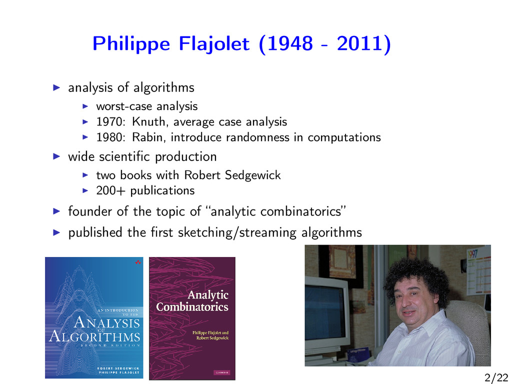
1970: Knuth, average case analysis 1980: Rabin, introduce randomness in computations wide scientific production two books with Robert Sedgewick 200+ publications founder of the topic of “analytic combinatorics” published the first sketching/streaming algorithms 2/22
over (also very large) domain D S = s1 s2 s3 · · · s , sj ∈ D consider S as a multiset M = m1 f1 m2 f2 · · · mn fn Interested in estimating the following quantitive statistics: — A. Length := — B. Cardinality := card(mi ) ≡ n (distinct values) ← this talk — C. Frequency moments := v∈D fv p p ∈ R Constraints: very little processing memory on the fly (single pass + simple main loop) no statistical hypothesis accuracy within a few percentiles 3/22
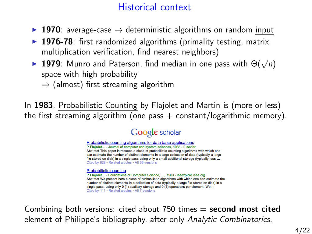
1976-78: first randomized algorithms (primality testing, matrix multiplication verification, find nearest neighbors) 1979: Munro and Paterson, find median in one pass with Θ( √ n) space with high probability ⇒ (almost) first streaming algorithm In 1983, Probabilistic Counting by Flajolet and Martin is (more or less) the first streaming algorithm (one pass + constant/logarithmic memory). Combining both versions: cited about 750 times = second most cited element of Philippe’s bibliography, after only Analytic Combinatorics. 4/22
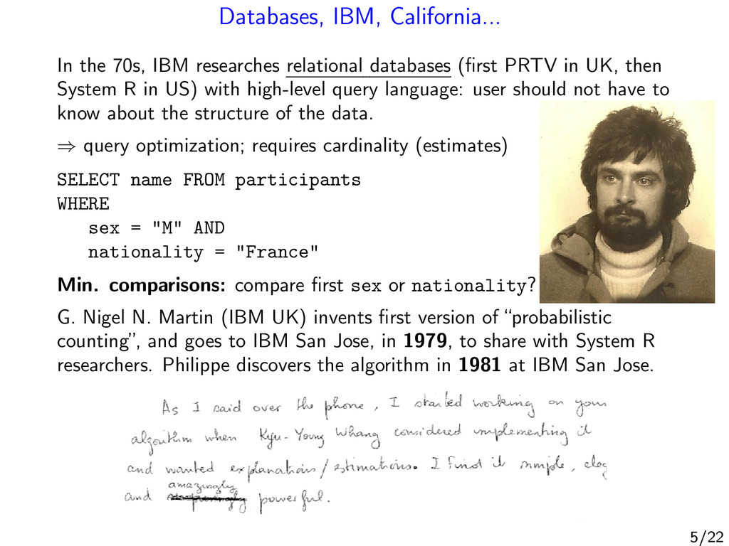
(first PRTV in UK, then System R in US) with high-level query language: user should not have to know about the structure of the data. ⇒ query optimization; requires cardinality (estimates) SELECT name FROM participants WHERE sex = "M" AND nationality = "France" Min. comparisons: compare first sex or nationality? G. Nigel N. Martin (IBM UK) invents first version of “probabilistic counting”, and goes to IBM San Jose, in 1979, to share with System R researchers. Philippe discovers the algorithm in 1981 at IBM San Jose. 5/22
tools for hash tables 1969: Bloom filters → first time in an approximate context 1977/79: Carter & Wegman, Universal Hashing, first time considered as probabilistic objects + proved uniformity is possible in practice hash functions transform data into i.i.d. uniform random variables or in infinite strings of random bits: h : D → {0, 1}∞ that is, if h(x) = b1 b2 · · · , then P[b1 = 1] = P[b2 = 1] = . . . = 1/2 Philippe’s approach was experimental later theoretically validated in 2010: Mitzenmacher & Vadhan proved hash functions “work” because they exploit the entropy of the hashed data 6/22
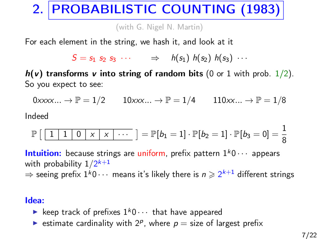
each element in the string, we hash it, and look at it S = s1 s2 s3 · · · ⇒ h(s1 ) h(s2 ) h(s3 ) · · · h(v) transforms v into string of random bits (0 or 1 with prob. 1/2). So you expect to see: 0xxxx... → P = 1/2 10xxx... → P = 1/4 110xx... → P = 1/8 Indeed P 1 1 0 x x · · · = P[b1 = 1] · P[b2 = 1] · P[b3 = 0] = 1 8 7/22
each element in the string, we hash it, and look at it S = s1 s2 s3 · · · ⇒ h(s1 ) h(s2 ) h(s3 ) · · · h(v) transforms v into string of random bits (0 or 1 with prob. 1/2). So you expect to see: 0xxxx... → P = 1/2 10xxx... → P = 1/4 110xx... → P = 1/8 Indeed P 1 1 0 x x · · · = P[b1 = 1] · P[b2 = 1] · P[b3 = 0] = 1 8 Intuition: because strings are uniform, prefix pattern 1k 0 · · · appears with probability 1/2k+1 ⇒ seeing prefix 1k 0 · · · means it’s likely there is n 2k+1 different strings Idea: keep track of prefixes 1k 0 · · · that have appeared estimate cardinality with 2p, where p = size of largest prefix 7/22
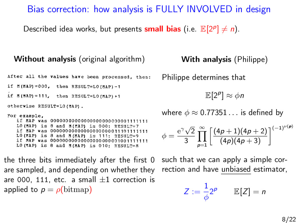
idea works, but presents small bias (i.e. E[2p] = n). Without analysis (original algorithm) the three bits immediately after the first 0 are sampled, and depending on whether they are 000, 111, etc. a small ±1 correction is applied to p = ρ(bitmap) With analysis (Philippe) Philippe determines that E[2p] ≈ φn where φ ≈ 0.77351 . . . is defined by φ = eγ √ 2 3 ∞ p=1 (4p + 1)(4p + 2) (4p)(4p + 3) (−1)ν(p) such that we can apply a simple cor- rection and have unbiased estimator, Z := 1 φ 2p E[Z] = n 8/22
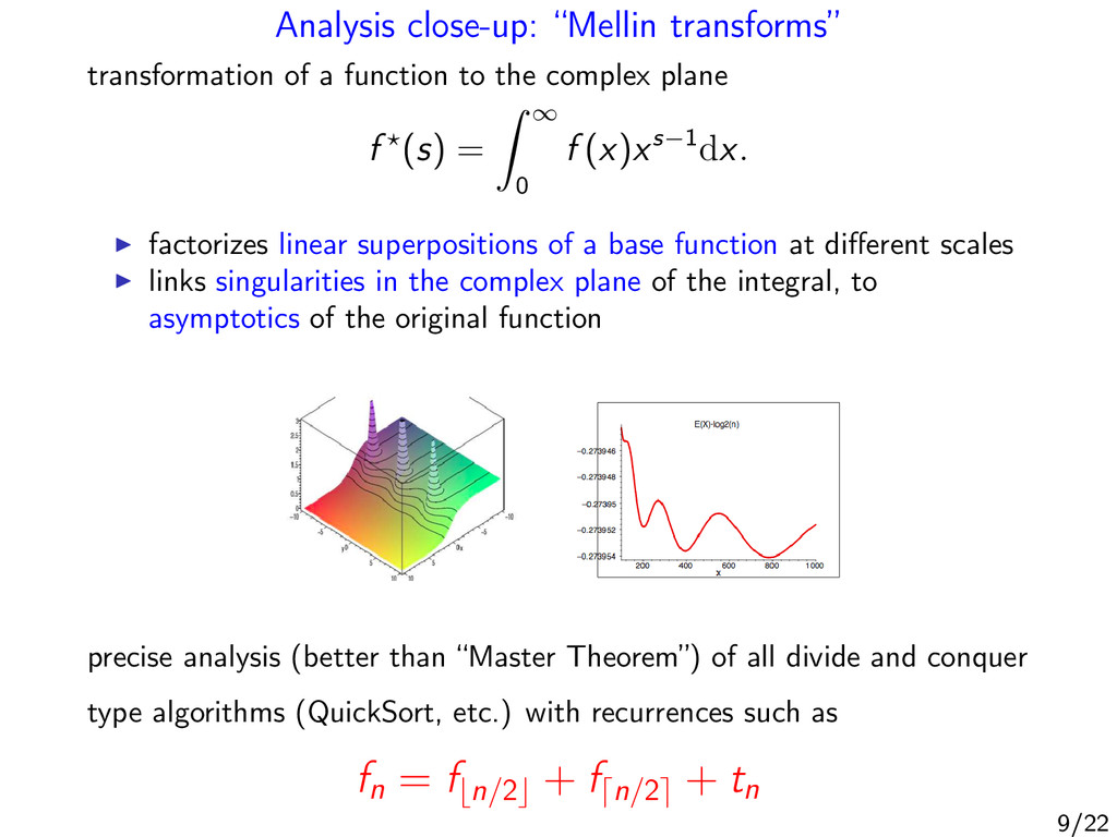
complex plane f (s) = ∞ 0 f (x)xs−1dx. factorizes linear superpositions of a base function at different scales links singularities in the complex plane of the integral, to asymptotics of the original function precise analysis (better than “Master Theorem”) of all divide and conquer type algorithms (QuickSort, etc.) with recurrences such as fn = f n/2 + f n/2 + tn 9/22
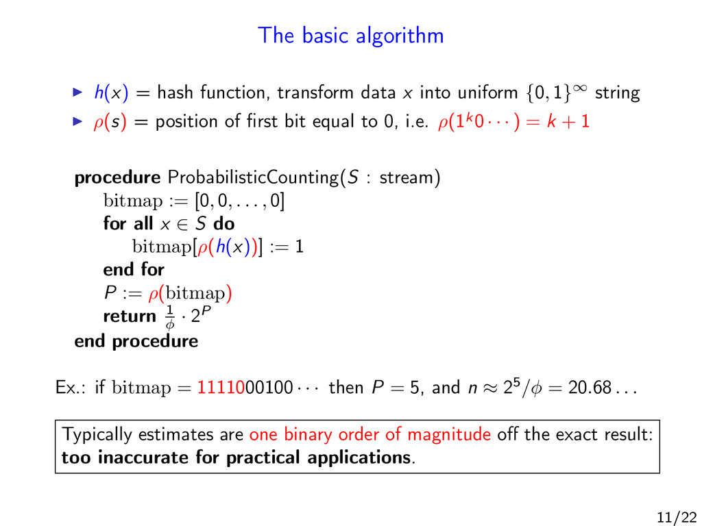
into uniform {0, 1}∞ string ρ(s) = position of first bit equal to 0, i.e. ρ(1k 0 · · · ) = k + 1 procedure ProbabilisticCounting(S : stream) bitmap := [0, 0, . . . , 0] for all x ∈ S do bitmap[ρ(h(x))] := 1 end for P := ρ(bitmap) return 1 φ · 2P end procedure Ex.: if bitmap = 1111000100 · · · then P = 5, and n ≈ 25/φ = 20.68 . . . Typically estimates are one binary order of magnitude off the exact result: too inaccurate for practical applications. 11/22
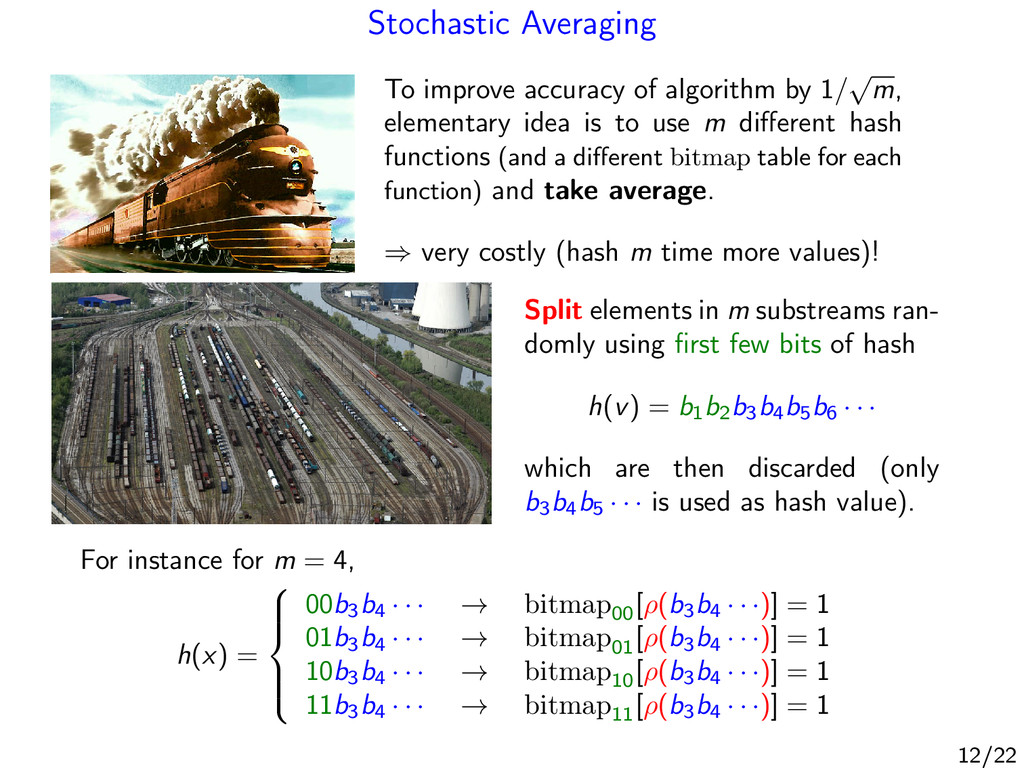
m, elementary idea is to use m different hash functions (and a different bitmap table for each function) and take average. ⇒ very costly (hash m time more values)! Split elements in m substreams ran- domly using first few bits of hash h(v) = b1 b2 b3 b4 b5 b6 · · · which are then discarded (only b3 b4 b5 · · · is used as hash value). For instance for m = 4, h(x) = 00b3 b4 · · · → bitmap00 [ρ(b3 b4 · · ·)] = 1 01b3 b4 · · · → bitmap01 [ρ(b3 b4 · · ·)] = 1 10b3 b4 · · · → bitmap10 [ρ(b3 b4 · · ·)] = 1 11b3 b4 · · · → bitmap11 [ρ(b3 b4 · · ·)] = 1 12/22
asymptotically unbiased estimator of cardinality, in the sense that En [Z] ∼ n and has accuracy using m bitmaps is σn [Z] n = 0.78 √ m Concretely, need O(m log n) memory (instead of O(n) for exact). Example: can count cardinalities up to n = 109 with error ±6%, using only 4096 bytes = 4 kB. 13/22
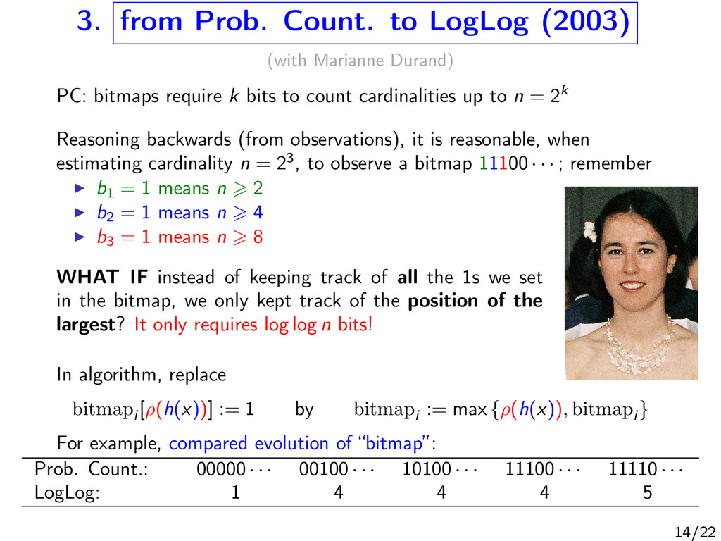
PC: bitmaps require k bits to count cardinalities up to n = 2k Reasoning backwards (from observations), it is reasonable, when estimating cardinality n = 23, to observe a bitmap 11100 · · · ; remember b1 = 1 means n 2 b2 = 1 means n 4 b3 = 1 means n 8 WHAT IF instead of keeping track of all the 1s we set in the bitmap, we only kept track of the position of the largest? It only requires log log n bits! In algorithm, replace bitmapi [ρ(h(x))] := 1 by bitmapi := max {ρ(h(x)), bitmapi } For example, compared evolution of “bitmap”: Prob. Count.: 00000 · · · 00100 · · · 10100 · · · 11100 · · · 11110 · · · LogLog: 1 4 4 4 5 14/22
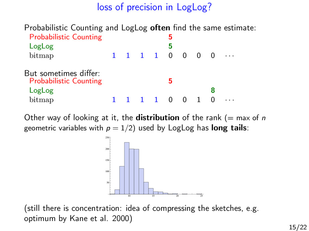
find the same estimate: Probabilistic Counting 5 LogLog 5 bitmap 1 1 1 1 0 0 0 0 · · · But sometimes differ: Probabilistic Counting 5 LogLog 8 bitmap 1 1 1 1 0 0 1 0 · · · Other way of looking at it, the distribution of the rank (= max of n geometric variables with p = 1/2) used by LogLog has long tails: 10 15 20 25 50 100 150 200 250 (still there is concentration: idea of compressing the sketches, e.g. optimum by Kane et al. 2000) 15/22
possible): Probabilistic Counting: 0.78/ √ m for m registers of 32 bits LogLog: 1.36/ √ m for m small registers of 5 bits In LogLog, loss of accuracy due to some (rare but real) registers that are too big, too far beyond the expected value. SuperLogLog is LogLog, in which we remove δ largest registers before estimating, i.e., δ = 70%. involves a two-time estimation analysis is much more complicated but accuracy much better: 1.05/ √ m 16/22
(2007) (with Eric Fusy, Frédéric Meunier & Olivier Gandouet) 2005: Giroire (PhD student of Philippe’s) publishes thesis with cardinality estimator based on order statistics 2006: Chassaing and Gerin, using statistical tools find best estimator based on order statistics in an information theoretic sense The note suggests using a harmonic mean: initially dismissed as a theoretical improvement, it turns out simulations are very good. Why? 18/22
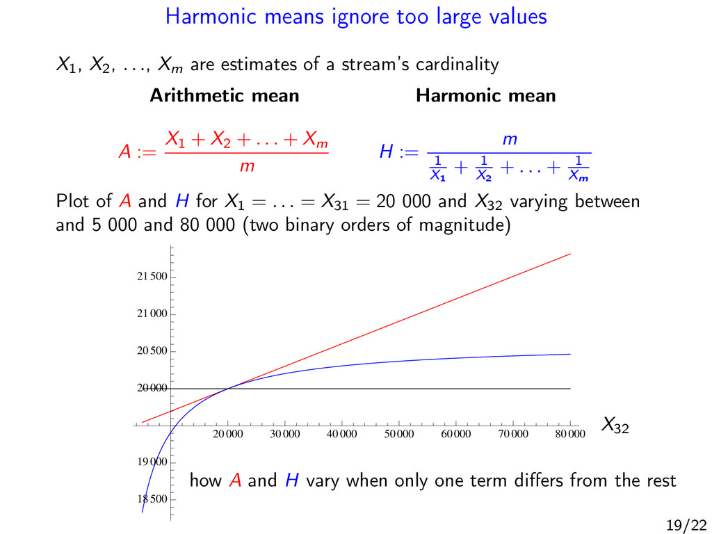
. . ., Xm are estimates of a stream’s cardinality Arithmetic mean Harmonic mean A := X1 + X2 + . . . + Xm m H := m 1 X1 + 1 X2 + . . . + 1 Xm Plot of A and H for X1 = . . . = X31 = 20 000 and X32 varying between and 5 000 and 80 000 (two binary orders of magnitude) how A and H vary when only one term differs from the rest X32 20000 30000 40000 50000 60000 70000 80000 18500 19000 20000 20500 21000 21500 19/22
as SuperLogLog, but substitutes algorithmic clev- erness with mathematical elegance. Accuracy is 1.03/ √ m with m small loglog bytes (≈ 4 bits). Whole of Shakespeare summarized: ghfffghfghgghggggghghheehfhfhhgghghghhfgffffhhhiigfhhffgfiihfhhh igigighfgihfffghigihghigfhhgeegeghgghhhgghhfhidiigihighihehhhfgg hfgighigffghdieghhhggghhfghhfiiheffghghihifgggffihgihfggighgiiif fjgfgjhhjiifhjgehgghfhhfhjhiggghghihigghhihihgiighgfhlgjfgjjjmfl Estimate ˜ n ≈ 30 897 against n = 28 239. Error is ±9.4% for 128 bytes. Pranav Kashyap: word-level encrypted texts, classification by language. 20/22
Counting, 1982: how to count up to n with only log log n memory a beautiful algorithm (with Wegman), Adaptive Sampling, 1989, which was ahead of its time, and was grossly unappreciated... until it was rediscovered in 2000: how do you count the number of elements which appear only once in a stream using constant size memory? 21/22
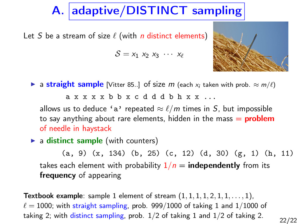
(with n distinct elements) S = x1 x2 x3 · · · x a straight sample [Vitter 85..] of size m (each xi taken with prob. ≈ m/ ) a x x x x b b x c d d d b h x x ... allows us to deduce ‘a’ repeated ≈ /m times in S, but impossible to say anything about rare elements, hidden in the mass = problem of needle in haystack a distinct sample (with counters) (a, 9) (x, 134) (b, 25) (c, 12) (d, 30) (g, 1) (h, 11) ( takes each element with probability 1/n = independently from its frequency of appearing Textbook example: sample 1 element of stream (1, 1, 1, 1, 2, 1, 1, . . . , 1), = 1000; with straight sampling, prob. 999/1000 of taking 1 and 1/1000 of taking 2; with distinct sampling, prob. 1/2 of taking 1 and 1/2 of taking 2. 22/22
![Theorem [FM85]. The estimator Z of Probabilistic Counting is an](https://files.speakerdeck.com/presentations/baddb7f0c0b1013039a5220f55e8ad8b/slide_13.jpg)