Sketching as a Tool for Numerical Linear Algebra

David Woodruff's talk at the AK Data Science Summit on Streaming and Sketching in Big Data and Analytics on 06/20/2013 at 111 Minna.

For more information: http://blog.aggregateknowledge.com/ak-data-science-summit-june-20-2013

Transcript

1. Sketching as a Tool for Numerical Linear Algebra David Woodruff IBM Almaden
2. 2 Massive data sets Examples §  Internet traffic logs §  Financial data §  etc. Algorithms §  Want nearly linear time or less §  Usually at the cost of a randomized approximation
3. 3 Regression analysis Regression §  Statistical method to study dependencies between variables in the presence of noise.
4. 4 Regression analysis Linear Regression §  Statistical method to study linear dependencies between variables in the presence of noise.
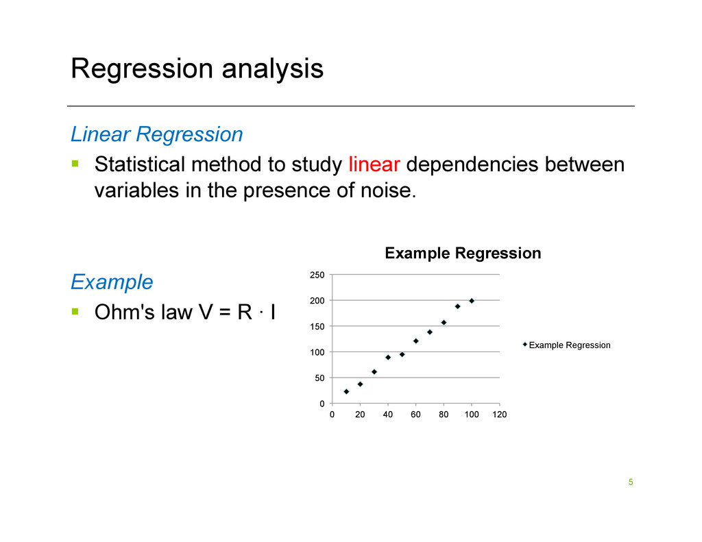
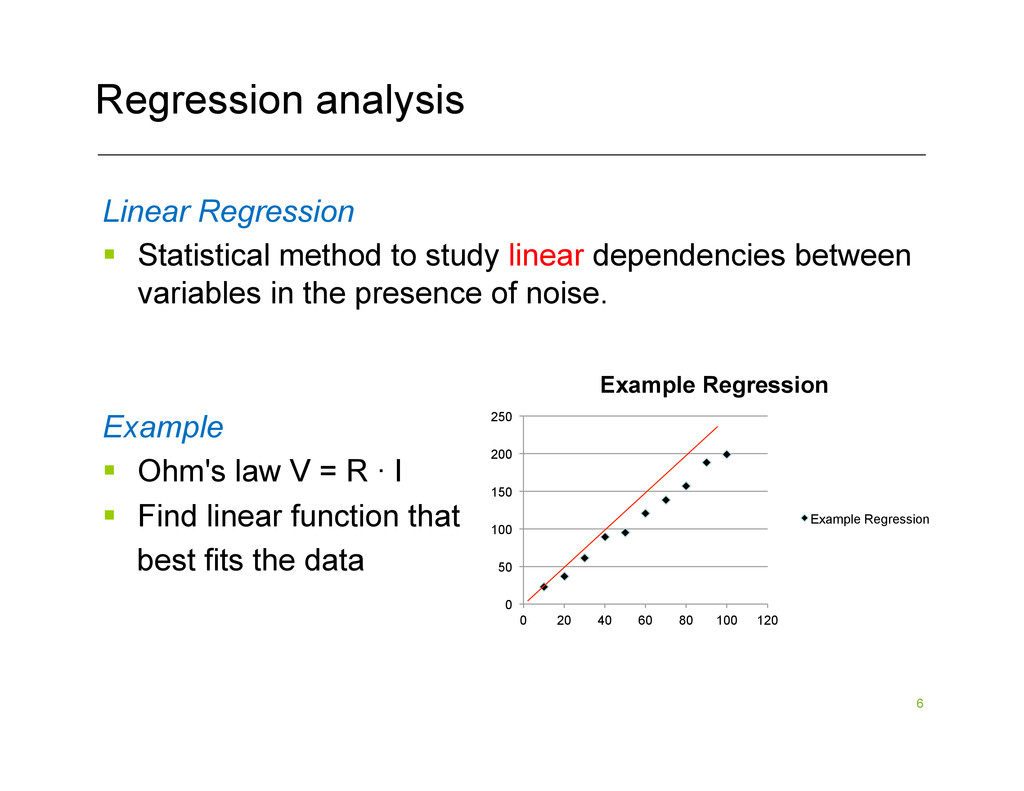
5. 5 Regression analysis Linear Regression §  Statistical method to study linear dependencies between variables in the presence of noise. Example §  Ohm's law V = R · I 0 50 100 150 200 250 0 20 40 60 80 100 120 Example Regression Example Regression
6. 6 Regression analysis Linear Regression §  Statistical method to study linear dependencies between variables in the presence of noise. Example §  Ohm's law V = R · I §  Find linear function that best fits the data 0 50 100 150 200 250 0 20 40 60 80 100 120 Example Regression Example Regression
7. 7 Regression analysis Linear Regression §  Statistical method to study linear dependencies between variables in the presence of noise. Standard Setting §  One measured variable b §  A set of predictor variables a ,…, a §  Assumption: b = x + a x + … + a x + ε §  ε is assumed to be noise and the xi are model parameters we want to learn §  Can assume x0 = 0 §  Now consider n measured variables 1 d 1 1 d d 0
8. 8 Regression analysis Matrix form Input: n×d-matrix A and a vector b=(b1 ,…, bn ) n is the number of observations; d is the number of predictor variables Output: x* so that Ax* and b are close §  Consider the over-constrained case, when n À d §  Can assume that A has full column rank
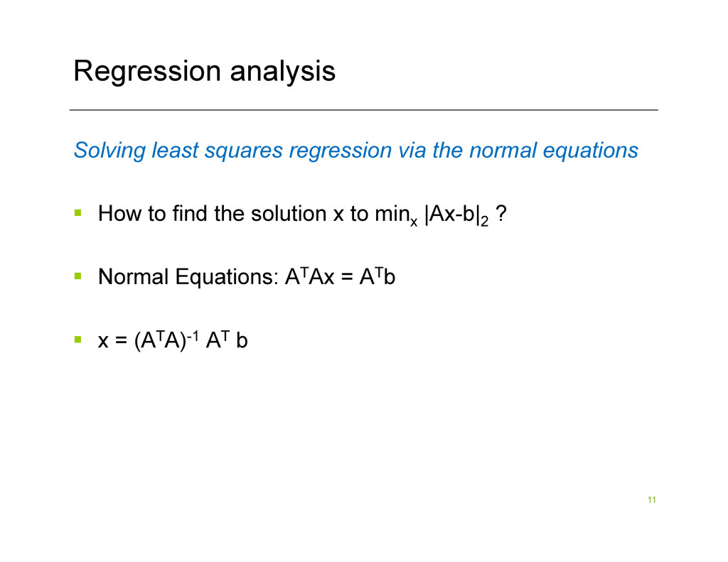
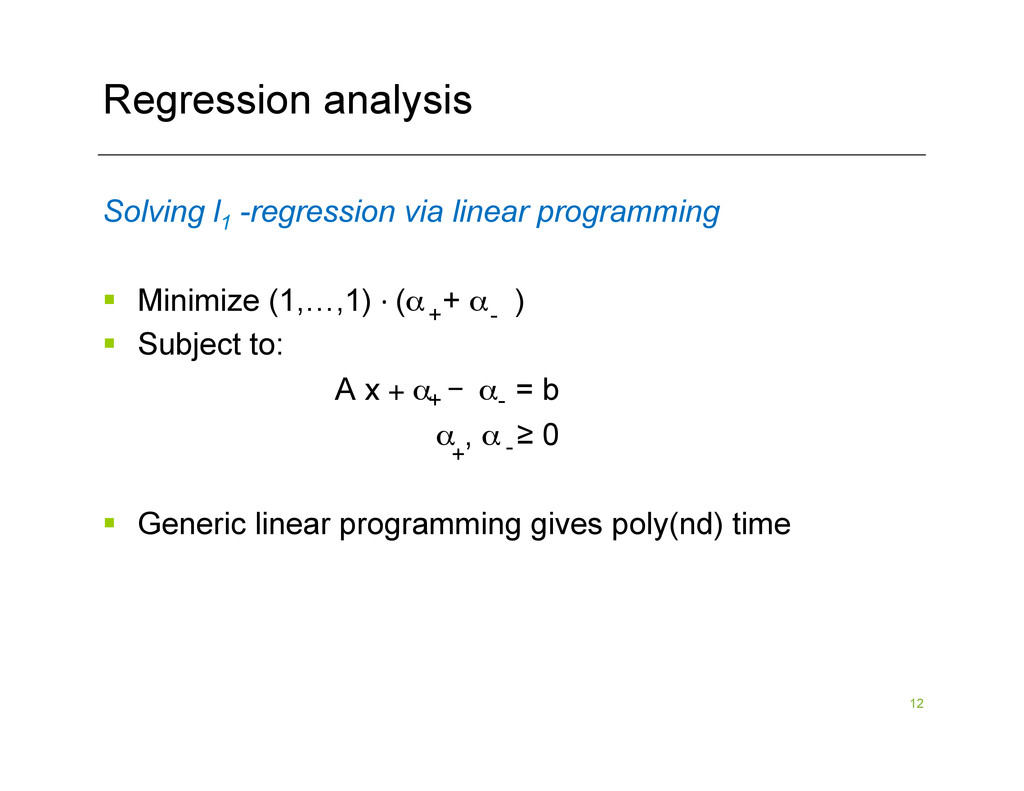
9. 9 Regression analysis Least Squares Method §  Find x* that minimizes |Ax-b|2 2 = Σ (bi – <Ai* , x>)² §  Ai* is i-th row of A §  Certain desirable statistical properties Method of least absolute deviation (l1 -regression) §  Find x* that minimizes |Ax-b|1 = Σ |bi – <Ai* , x>| §  Cost is less sensitive to outliers than least squares
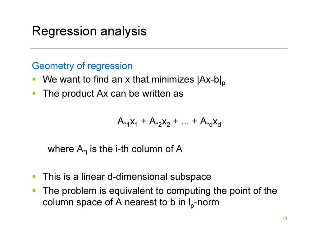
10. 10 Regression analysis Geometry of regression §  We want to find an x that minimizes |Ax-b|p §  The product Ax can be written as A*1 x1 + A*2 x2 + ... + A*d xd where A*i is the i-th column of A §  This is a linear d-dimensional subspace §  The problem is equivalent to computing the point of the column space of A nearest to b in lp -norm
11. 11 Regression analysis Solving least squares regression via the normal equations §  How to find the solution x to minx |Ax-b|2 ? §  Normal Equations: ATAx = ATb §  x = (ATA)-1 AT b
12. 12 Regression analysis Solving l1 -regression via linear programming §  Minimize (1,…,1) ·∙  (α + α ) §  Subject to: A x + α - α = b α , α ≥ 0 §  Generic linear programming gives poly(nd) time + - + - + -
13. 13 Talk Outline §  Sketching to speed up Least Squares Regression §  Sketching to speed up Least Absolute Deviation (l1 ) Regression §  Sketching to speed up Low Rank Approximation
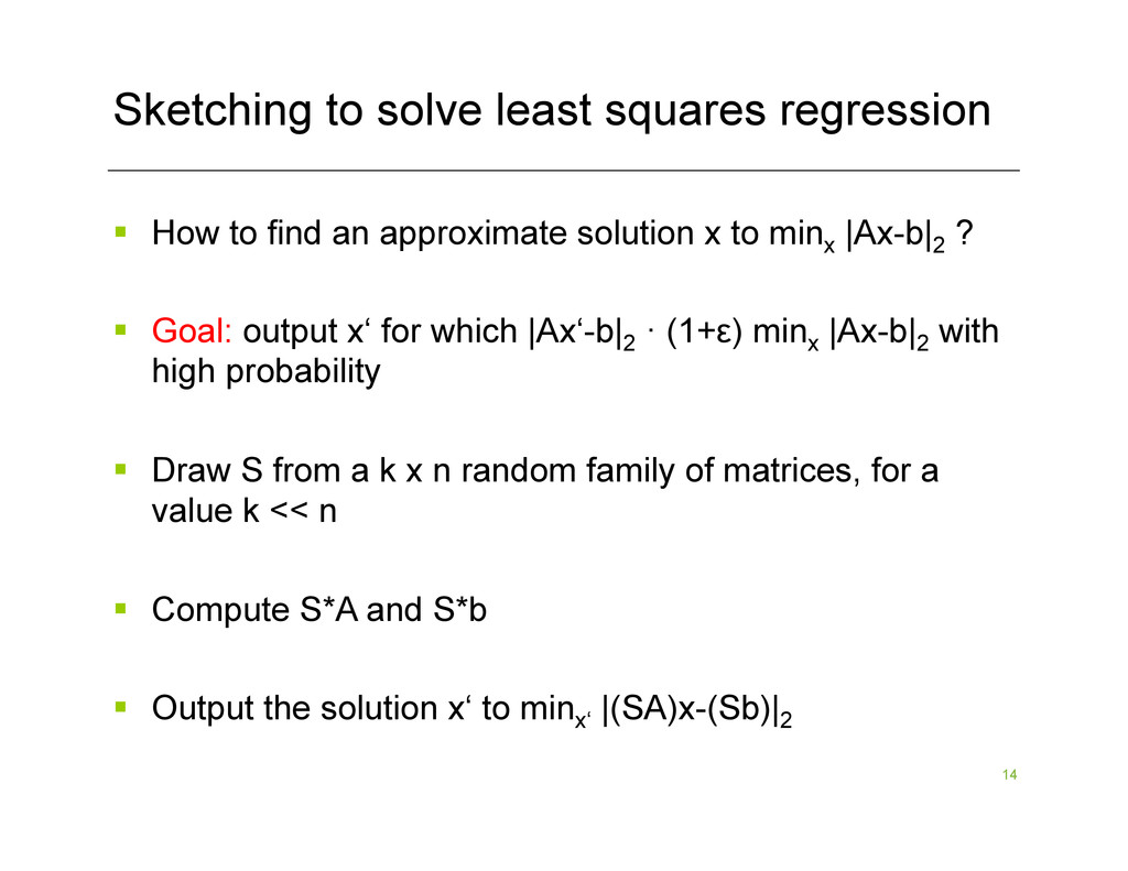
14. 14 Sketching to solve least squares regression §  How to find an approximate solution x to minx |Ax-b|2 ? §  Goal: output x‘ for which |Ax‘-b|2 · (1+ε) minx |Ax-b|2 with high probability §  Draw S from a k x n random family of matrices, for a value k << n §  Compute S*A and S*b §  Output the solution x‘ to minx‘ |(SA)x-(Sb)|2
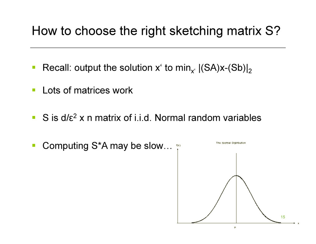
15. 15 How to choose the right sketching matrix S? §  Recall: output the solution x‘ to minx‘ |(SA)x-(Sb)|2 §  Lots of matrices work §  S is d/ε2 x n matrix of i.i.d. Normal random variables §  Computing S*A may be slow…
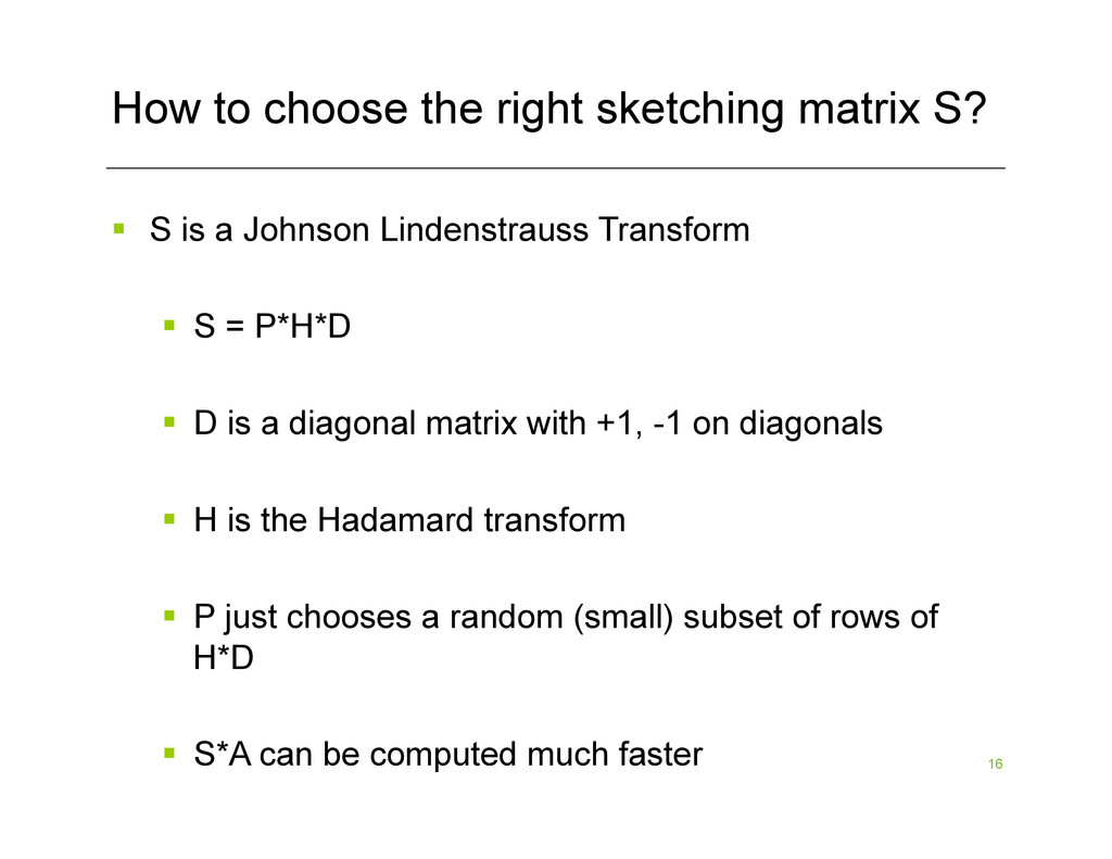
16. 16 How to choose the right sketching matrix S? §  S is a Johnson Lindenstrauss Transform §  S = P*H*D §  D is a diagonal matrix with +1, -1 on diagonals §  H is the Hadamard transform §  P just chooses a random (small) subset of rows of H*D §  S*A can be computed much faster
17. 17 Even faster sketching matrices S [ [ 0 0 1 0 0 1 0 0 1 0 0 0 0 0 0 0 0 0 0 -1 1 0 -1 0 0-1 0 0 0 0 0 1 §  CountSketch matrix §  Define k x n matrix S, for k = d2/ε2 §  S is really sparse: single randomly chosen non-zero entry per column Surprisingly, this works!
18. 18 Talk Outline §  Sketching to speed up Least Squares Regression §  Sketching to speed up Least Absolute Deviation (l1 ) Regression §  Sketching to speed up Low Rank Approximation
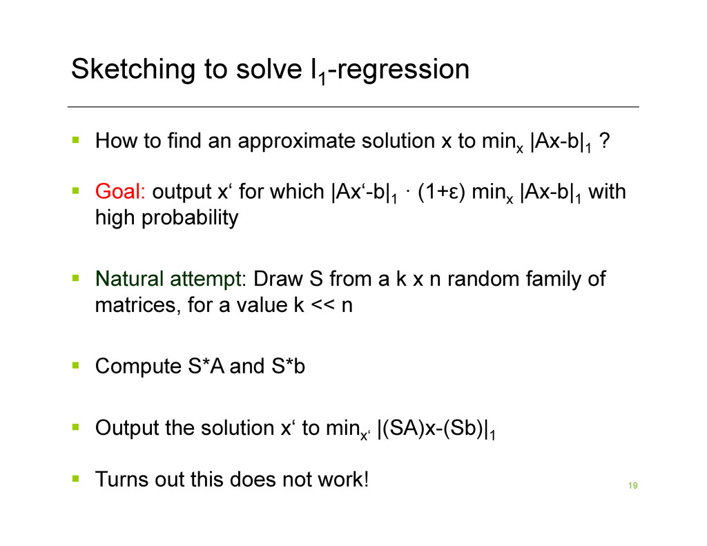
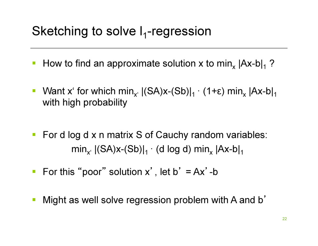
19. 19 Sketching to solve l1 -regression §  How to find an approximate solution x to minx |Ax-b|1 ? §  Goal: output x‘ for which |Ax‘-b|1 · (1+ε) minx |Ax-b|1 with high probability §  Natural attempt: Draw S from a k x n random family of matrices, for a value k << n §  Compute S*A and S*b §  Output the solution x‘ to minx‘ |(SA)x-(Sb)|1 §  Turns out this does not work!
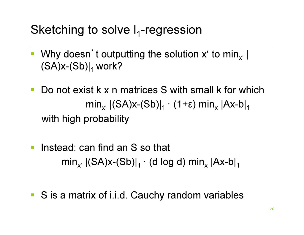
20. 20 Sketching to solve l1 -regression §  Why doesn’t outputting the solution x‘ to minx‘ | (SA)x-(Sb)|1 work? §  Do not exist k x n matrices S with small k for which minx‘ |(SA)x-(Sb)|1 · (1+ε) minx |Ax-b|1 with high probability §  Instead: can find an S so that minx‘ |(SA)x-(Sb)|1 · (d log d) minx |Ax-b|1 §  S is a matrix of i.i.d. Cauchy random variables
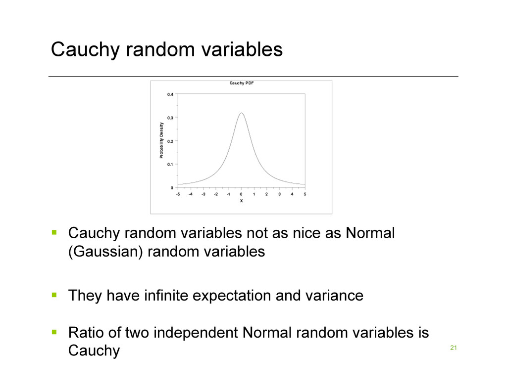
21. 21 Cauchy random variables §  Cauchy random variables not as nice as Normal (Gaussian) random variables §  They have infinite expectation and variance §  Ratio of two independent Normal random variables is Cauchy
22. 22 Sketching to solve l1 -regression §  How to find an approximate solution x to minx |Ax-b|1 ? §  Want x‘ for which minx‘ |(SA)x-(Sb)|1 · (1+ε) minx |Ax-b|1 with high probability §  For d log d x n matrix S of Cauchy random variables: minx‘ |(SA)x-(Sb)|1 · (d log d) minx |Ax-b|1 §  For this “poor” solution x’, let b’ = Ax’-b §  Might as well solve regression problem with A and b’
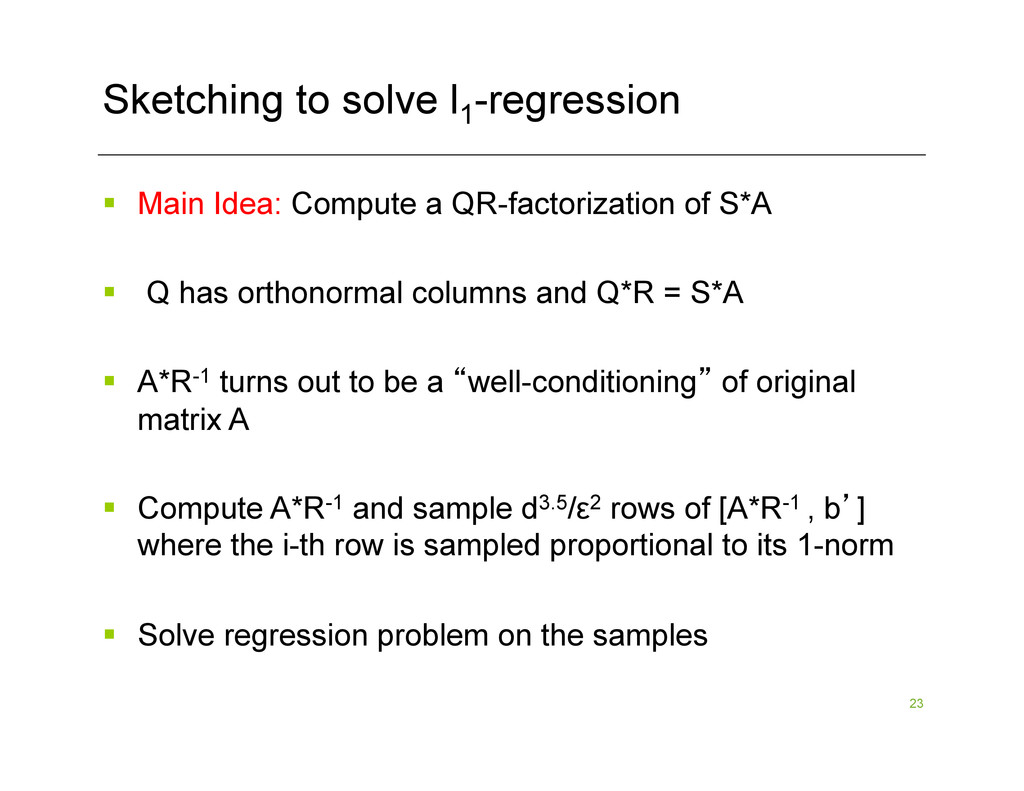
23. 23 Sketching to solve l1 -regression §  Main Idea: Compute a QR-factorization of S*A §  Q has orthonormal columns and Q*R = S*A §  A*R-1 turns out to be a “well-conditioning” of original matrix A §  Compute A*R-1 and sample d3.5/ε2 rows of [A*R-1 , b’] where the i-th row is sampled proportional to its 1-norm §  Solve regression problem on the samples
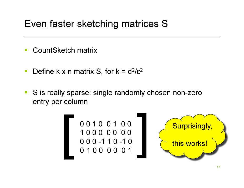
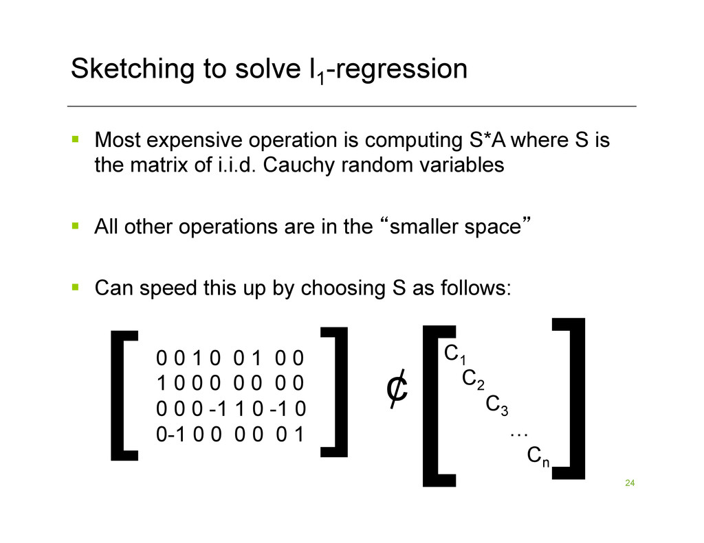
24. 24 Sketching to solve l1 -regression §  Most expensive operation is computing S*A where S is the matrix of i.i.d. Cauchy random variables §  All other operations are in the “smaller space” §  Can speed this up by choosing S as follows: [ [ 0 0 1 0 0 1 0 0 1 0 0 0 0 0 0 0 0 0 0 -1 1 0 -1 0 0-1 0 0 0 0 0 1 ¢ [ [C1 C2 C3 … Cn
25. 25 Further sketching improvements §  Can show you need a fewer number of sampled rows in later steps if instead choose S as follows §  Instead of diagonal of Cauchy random variables, choose diagonal of reciprocals of exponential random variables [ [ 0 0 1 0 0 1 0 0 1 0 0 0 0 0 0 0 0 0 0 -1 1 0 -1 0 0-1 0 0 0 0 0 1 ¢ [ [1/E1 1/E2 1/E3 … 1/En
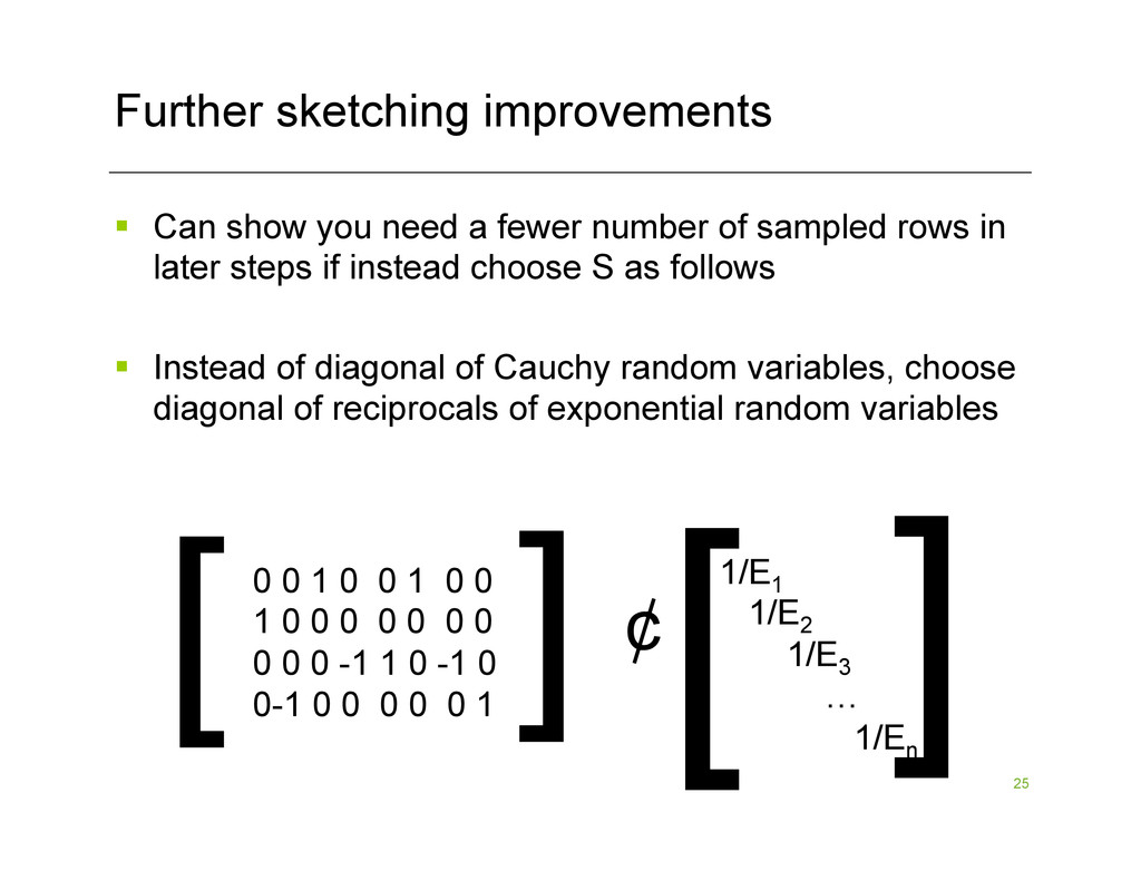
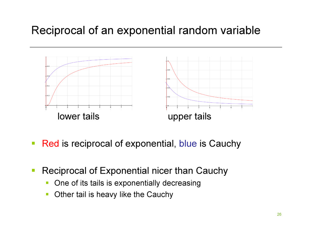
26. 26 Reciprocal of an exponential random variable lower tails upper tails §  Red is reciprocal of exponential, blue is Cauchy §  Reciprocal of Exponential nicer than Cauchy §  One of its tails is exponentially decreasing §  Other tail is heavy like the Cauchy
27. 27 Talk Outline §  Sketching to speed up Least Squares Regression §  Sketching to speed up Least Absolute Deviation (l1 ) Regression §  Sketching to speed up Low Rank Approximation
28. 28 Low rank approximation §  A is an n x n matrix §  Typically well-approximated by low rank matrix §  E.g., only high rank because of noise §  Want to output a rank k matrix A’, so that |A-A’|F · (1+ε) |A-Ak | F , w.h.p., where Ak = argminrank k matrices B |A-B|F §  For matrix C, |C|F = (Σi,j Ci,j 2)1/2
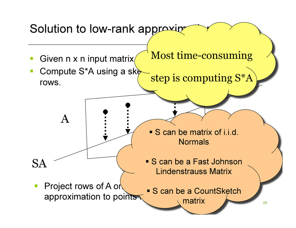
29. 29 Solution to low-rank approximation §  Given n x n input matrix A §  Compute S*A using a sketching matrix S with k << n rows. SA A §  Project rows of A onto SA, then find best rank-k approximation to points inside of SA Most time-consuming step is computing S*A §  S can be matrix of i.i.d. Normals §  S can be a Fast Johnson Lindenstrauss Matrix §  S can be a CountSketch matrix
30. 30 Caveat: projecting the points onto SA is slow §  Current algorithm: 1. Compute S*A (easy) 2. Project each of the rows onto S*A 3. Find best rank-k approximation of projected points inside of rowspace of S*A (easy) §  Bottleneck is step 2 §  Turns out if you compute (AR)(S*A*R)-(SA), this is a good low-rank approximation
31. 31 Conclusion §  Gave fast sketching-based algorithms for numerical linear algebra problems §  Least Squares Regression §  Least Absolute Deviation (l1 ) Regression §  Low Rank Approximation §  Sketching also provides “dimensionality reduction” §  Communication-efficient solutions for these problems