Defense Presentation (Tanay)

Transcript

1. Latent Representation and Sampling in Network: Application in Text Mining and Biology Tanay Kumar Saha Purdue University, West Lafayette, Indiana, USA April 9, 2018 Tanay Kumar Saha (Defense Presentation) Latent Representation and Sampling April 9, 2018 1 / 58
2. Outline 1 About Me 2 Thesis Contribution 3 Introduction and Motivation Data Representation 4 Our Approach for Modeling Temporal Smoothness in an Evolving Network Modeling Temporal Smoothness Solution Sketch Mathematical Formulation 5 Our Approach for Learning Sentence Representation Latent Representation of Sentences Description of Models Evaluation 6 Frequent Subgraph Mining Details of the Methods Some Results 7 Conclusion Tanay Kumar Saha (Defense Presentation) Latent Representation and Sampling April 9, 2018 2 / 58
3. About Me PhD Start Date: August 2012 (Collab:QCRI, NEC labs, eBay, CareerBuilder, iControlESI) Problem/Areas Worked: (1) Latent Representation in Networks, (2) Network Sampling, (3) Total Recall, (4) Name Disambiguation Already Published: ECML/PKDD(1), CIKM (1), TCBB (1), SADM (1), SNAM (1), IEEE Big Data (1), ASONAM (1), Complenet (1), IEEE CNS (1), BIOKDD (1) Poster Presentation: RECOMB (1), IEEE Big Data (1) Paper Under Review: KDD (1), JBHI (1), TMC(1) In Preparation: ECML/PKDD(1), CIKM(1) Reproducible Research: Released codes for all the works related to the thesis Served as a Reviewer: TKDE, TOIS Provisional Patent Application (3) Apparatus and Method of Implementing Batch-mode active learning for Technology-Assisted Review (iControlESI) Apparatus and Method of Implementing Enhanced Batch-Mode Active Learning for Technology-Assisted Review of Documents (iControlESI) Method and System for Log Based Computer Server Failure Diagnosis (NEC Labs) Tanay Kumar Saha (Defense Presentation) Latent Representation and Sampling April 9, 2018 3 / 58
4. Outline 1 About Me 2 Thesis Contribution 3 Introduction and Motivation Data Representation 4 Our Approach for Modeling Temporal Smoothness in an Evolving Network Modeling Temporal Smoothness Solution Sketch Mathematical Formulation 5 Our Approach for Learning Sentence Representation Latent Representation of Sentences Description of Models Evaluation 6 Frequent Subgraph Mining Details of the Methods Some Results 7 Conclusion Tanay Kumar Saha (Defense Presentation) Latent Representation and Sampling April 9, 2018 4 / 58
5. Thesis Contribution Before Proposal After Proposal Latent Representation and Sampling in Networks Latent Representation Sampling and Its Applications Frequent Subgraph Mining IEEE Big Data (2014), SADM (2015)) Motif Finding Complenet (2015) Android App Classification IEEE CNS (2016), IEEE TMC (2018)
6. Thesis Contribution Before Proposal After Proposal Latent Representation and Sampling in Networks Latent Representation Sampling and Its Applications Frequent Subgraph Mining IEEE Big Data (2014), SADM (2015)) Motif Finding Complenet (2015) Android App Classification IEEE CNS (2016), IEEE TMC (2018) Latent Representation of Nodes in Evolving Network KDD (2018) Latent Representation of Edges in Evolving Network MLJ (2018) Retrofitted and Regular- ized Models for Latent Representation of Sentences CIKM (2017) Joint Model for Sentence Representation ECML-PKDD (2017) Functional Motif Detection TCBB (2017) Tanay Kumar Saha (Defense Presentation) Latent Representation and Sampling April 9, 2018 5 / 58
7. Outline 1 About Me 2 Thesis Contribution 3 Introduction and Motivation Data Representation 4 Our Approach for Modeling Temporal Smoothness in an Evolving Network Modeling Temporal Smoothness Solution Sketch Mathematical Formulation 5 Our Approach for Learning Sentence Representation Latent Representation of Sentences Description of Models Evaluation 6 Frequent Subgraph Mining Details of the Methods Some Results 7 Conclusion Tanay Kumar Saha (Defense Presentation) Latent Representation and Sampling April 9, 2018 6 / 58
8. Data Representation For machine learning algorithms, we may need to represent data in the d-dimensional space Tanay Kumar Saha (Defense Presentation) Latent Representation and Sampling April 9, 2018 7 / 58
9. Data Representation For machine learning algorithms, we may need to represent data in the d-dimensional space For link prediction in network, we may represent edges in the space of total number of nodes in a network (d = |V |) Network Repre. of Nodes Repre. of Edges 1 2 3 4 5 id V1 V2 V3 · · · V1 0 1 1 · · · V2 1 0 1 · · · id V1 V2 V3 · · · V1-V2 0 0 1 · · · Tanay Kumar Saha (Defense Presentation) Latent Representation and Sampling April 9, 2018 7 / 58
10. Data Representation For machine learning algorithms, we may need to represent data in the d-dimensional space For link prediction in network, we may represent edges in the space of total number of nodes in a network (d = |V |) Network Repre. of Nodes Repre. of Edges 1 2 3 4 5 id V1 V2 V3 · · · V1 0 1 1 · · · V2 1 0 1 · · · id V1 V2 V3 · · · V1-V2 0 0 1 · · · For document summarization, we may represent a particular sentence in the space of vocabulary/word size (d = |W|) Sentence Representation Sent id Content w1 w2 w3 · · · S1 This place is nice 1 0 1 · · · S2 This place is beautiful 1 1 0 · · · Tanay Kumar Saha (Defense Presentation) Latent Representation and Sampling April 9, 2018 7 / 58
11. Data Representation in the Latent Space From discrete to continuous space Capture syntactic (homophily) and semantic (structural equivalence) properties of textual (words, sentences) and network units (nodes, edges) Tanay Kumar Saha (Defense Presentation) Latent Representation and Sampling April 9, 2018 8 / 58
12. Data Representation in the Latent Space From discrete to continuous space Capture syntactic (homophily) and semantic (structural equivalence) properties of textual (words, sentences) and network units (nodes, edges) For link prediction in network, we may represent edges as a fixed-length vector Network Repre. of Nodes Repre. of Edges 1 2 3 4 5 id a1 a2 a3 V1 0.2 0.3 0.1 V2 0.1 0.2 0.3 id a1 a2 a3 V1-V2 0.02 0.06 0.03 Tanay Kumar Saha (Defense Presentation) Latent Representation and Sampling April 9, 2018 8 / 58
13. Data Representation in the Latent Space From discrete to continuous space Capture syntactic (homophily) and semantic (structural equivalence) properties of textual (words, sentences) and network units (nodes, edges) For link prediction in network, we may represent edges as a fixed-length vector Network Repre. of Nodes Repre. of Edges 1 2 3 4 5 id a1 a2 a3 V1 0.2 0.3 0.1 V2 0.1 0.2 0.3 id a1 a2 a3 V1-V2 0.02 0.06 0.03 Also for document summarization, we may represent a particular sentence as a fixed-length vector (say, 3-dimensional space) Sentence Representation Sent id Content a1 a2 a3 S1 This place is nice 0.2 0.3 0.4 S2 This place is beautiful 0.2 0.3 0.4 Tanay Kumar Saha (Defense Presentation) Latent Representation and Sampling April 9, 2018 8 / 58
14. Data Representation Project PAI Example from Pinterest Echo, Siri Tanay Kumar Saha (Defense Presentation) Latent Representation and Sampling April 9, 2018 9 / 58
15. Data Representation Network Repre. of Nodes Repre. of Edges 1 2 3 4 5 id a1 a2 a3 V1 0.2 0.3 0.1 V2 0.1 0.2 0.3 id a1 a2 a3 V1-V2 0.02 0.06 0.03 A problem with the abstract features that we learn is that they lack interpretability (What does a1 represent?) In real-life applications on network data, for some tasks, it is crucial to learn interpretable features in the form of graphical structures (fixed size substructures) For this we need to mine important graphical structures along with their frequency statistics from the input dataset The graphical structures may be necessary to induce structural information in the representation learning process Tanay Kumar Saha (Defense Presentation) Latent Representation and Sampling April 9, 2018 10 / 58
16. Data Representation (Frequent Subgraph Mining) A B F C D D A D B E C B E D G1 G2 G3 Given a set of networks, such as G1, G2, and G3 Tanay Kumar Saha (Defense Presentation) Latent Representation and Sampling April 9, 2018 11 / 58
17. Data Representation (Frequent Subgraph Mining) A B F C D D A D B E C B E D G1 G2 G3 Given a set of networks, such as G1, G2, and G3 Find frequent subgraphs of different sizes A B B C B D B E D E 2-node frequent subgraphs Tanay Kumar Saha (Defense Presentation) Latent Representation and Sampling April 9, 2018 11 / 58
18. Data Representation (Frequent Subgraph Mining) A B F C D D A D B E C B E D G1 G2 G3 Given a set of networks, such as G1, G2, and G3 Find frequent subgraphs of different sizes A B B C B D B E D E 2-node frequent subgraphs D B E A B C A B D B D E B E D C B D B D E 3-node frequent subgraphs Tanay Kumar Saha (Defense Presentation) Latent Representation and Sampling April 9, 2018 11 / 58
19. Data Representation (Frequent Subgraph Mining) A B F C D D A D B E C B E D G1 G2 G3 Given a set of networks, such as G1, G2, and G3 Find frequent subgraphs of different sizes A B B C B D B E D E 2-node frequent subgraphs D B E A B C A B D B D E B E D C B D B D E 3-node frequent subgraphs A B C D 4-node frequent subgraphs Tanay Kumar Saha (Defense Presentation) Latent Representation and Sampling April 9, 2018 11 / 58
20. Data Representation (Frequent Subgraph Mining) A B F C D D A D B E C B E D G1 G2 G3 Given a set of networks, such as G1, G2, and G3 Find frequent subgraphs of different sizes A B B C B D B E D E 2-node frequent subgraphs A B C B D E 3-node frequent subgraphs Induced Subgraphs Tanay Kumar Saha (Defense Presentation) Latent Representation and Sampling April 9, 2018 11 / 58
21. Data Representation (Frequent Subgraph Mining) A B F C D D A D B E C B E D G1 G2 G3 Given a set of networks, such as G1, G2, and G3 Find frequent subgraphs of different sizes Mining Steps: Candidate Generation, Subgraph Isomorphism checking, and Storing Candidates Tanay Kumar Saha (Defense Presentation) Latent Representation and Sampling April 9, 2018 11 / 58
22. Data Representation (Frequent Subgraph Mining) Table: Highlights of the lack of scalability of existing frequent subgraph mining methods while mining the PS dataset. Time indicates the running time of the fastest version of Gaston [Nijssen.Kok] Dataset Statistics: # graphs: 90, avg. # vertices: 67, avg. # edges: 268 # node labels: 20, # edge labels: 3 Time vs Max. subgraph size Time vs different minsup Search Space vs subgraph size (min-sup is fixed at 40%) (Max-size is fixed at 8) Max-size Time
23. Data Representation (Frequent Subgraph Mining) Table: Highlights of the lack of scalability of existing frequent subgraph mining methods while mining the PS dataset. Time indicates the running time of the fastest version of Gaston [Nijssen.Kok] Dataset Statistics: # graphs: 90, avg. # vertices: 67, avg. # edges: 268 # node labels: 20, # edge labels: 3 Time vs Max. subgraph size Time vs different minsup Search Space vs subgraph size (min-sup is fixed at 40%) (Max-size is fixed at 8) Max-size Time Support Time (%) 28 1.1 hours 22 3.5 hours 17 9 hours 11 >16 hours
24. Data Representation (Frequent Subgraph Mining) Table: Highlights of the lack of scalability of existing frequent subgraph mining methods while mining the PS dataset. Time indicates the running time of the fastest version of Gaston [Nijssen.Kok] Dataset Statistics: # graphs: 90, avg. # vertices: 67, avg. # edges: 268 # node labels: 20, # edge labels: 3 Time vs Max. subgraph size Time vs different minsup Search Space vs subgraph size (min-sup is fixed at 40%) (Max-size is fixed at 8) Max-size Time Support Time Size Induced Subgraph (%) Count 28 1.1 hours 6 26 millions 22 3.5 hours 7 157 millions 17 9 hours 8 947 millions 11 >16 hours 9 5000 billions
25. Data Representation (Frequent Subgraph Mining) Table: Highlights of the lack of scalability of existing frequent subgraph mining methods while mining the PS dataset. Time indicates the running time of the fastest version of Gaston [Nijssen.Kok] Dataset Statistics: # graphs: 90, avg. # vertices: 67, avg. # edges: 268 # node labels: 20, # edge labels: 3 Time vs Max. subgraph size Time vs different minsup Search Space vs subgraph size (min-sup is fixed at 40%) (Max-size is fixed at 8) Max-size Time Support Time Size Induced Subgraph (%) Count 8 6 minutes 28 1.1 hours 6 26 millions 9 2.8 hours 22 3.5 hours 7 157 millions 10 > 1.5 days 17 9 hours 8 947 millions 11 >16 hours 9 5000 billions Tanay Kumar Saha (Defense Presentation) Latent Representation and Sampling April 9, 2018 12 / 58
26. Data Representation (FSM Application) We propose FS3, which is a sampling based method and scalable FS3 performs a Markov Chain Monte Carlo (MCMC) sampling over the space of a fixed-size subgraphs We show application of our algorithm in biological network strucures such as, HIV and TIM (a) HIV (b) TIM Tanay Kumar Saha (Defense Presentation) Latent Representation and Sampling April 9, 2018 13 / 58
27. Data Representation (Frequent subgraph Mining) Given a single large undirected network, find the concentration of 3, 4, and 5-size graphlets 3-node subgraph patterns 4-node subgraph patterns 5-node subgraph patterns Figure: All 3, 4 and 5 node topologies Tanay Kumar Saha (Defense Presentation) Latent Representation and Sampling April 9, 2018 14 / 58
28. Data Representation (Frequent subgraph Mining) Given a single large directed network, find the concentration of 3, 4, and 5-size directed graphlets ω3 , 1 ω3 , 2 ω3 , 3 ω3 , 4 ω3 , 5 ω3 , 6 ω3 , 7 ω3 , 8 ω3 , 9 ω3 , 10 ω3 , 11 ω3 , 12 ω3 , 13 Figure: The 13 unique 3-graphlet types ω3,i (i = 1, 2, . . . , 13). Tanay Kumar Saha (Defense Presentation) Latent Representation and Sampling April 9, 2018 15 / 58
29. Data Representation (FSM Application (2)) We propose MHRW algorithm for finding the concentration of both the directed and undirected graphlet We show application in biology and security domain 0.45� 0.38� 0.35� 0.19� 0.16� Figure: The top 5 most frequent graphlet types for benign apps, i.e., the ones that have the highest average graphlet frequency densities across all benign apps. 0.52� 0.31� 0.26� 0.19� 0.19� Figure: The top 5 most frequent graphlet types for malware, i.e., the ones that have the highest average graphlet frequency densities across all malware. Tanay Kumar Saha (Defense Presentation) Latent Representation and Sampling April 9, 2018 16 / 58
30. Outline 1 About Me 2 Thesis Contribution 3 Introduction and Motivation Data Representation 4 Our Approach for Modeling Temporal Smoothness in an Evolving Network Modeling Temporal Smoothness Solution Sketch Mathematical Formulation 5 Our Approach for Learning Sentence Representation Latent Representation of Sentences Description of Models Evaluation 6 Frequent Subgraph Mining Details of the Methods Some Results 7 Conclusion Tanay Kumar Saha (Defense Presentation) Latent Representation and Sampling April 9, 2018 17 / 58
31. Data Representation Network Repre. of Nodes Repre. of Edges 1 2 3 4 5 id V1 V2 V3 · · · V1 0 1 1 · · · V2 1 0 1 · · · id V1 V2 V3 · · · V1-V2 0 0 1 · · · For Networks, we may also collect/hand-craft various kinds of features Node features: Degree, Closeness, Betweenness centrality Edge features: Common neighbor, Adamic-Adar Higher order features: Graphlet statistics, Frequent subgraph statistics Assumption: Networks are static In real-life, Networks are not static In social network, relationship among people changes over time Anatomical activity among the regions of human brain is also not static rather dynamic in nature Tanay Kumar Saha (Defense Presentation) Latent Representation and Sampling April 9, 2018 18 / 58
32. Static vs Dynamic (Evolving) Network Static: A Single snapshot of a network at a particular time-stamp 4 1 3 2 5 G1 Figure: A Toy Evolving Network. G1 , G2 and G3 are three snapshots of the Network.
33. Static vs Dynamic (Evolving) Network Static: A Single snapshot of a network at a particular time-stamp 4 1 3 2 5 G1 4 1 3 2 5 G2 4 1 3 2 5 G3 Figure: A Toy Evolving Network. G1 , G2 and G3 are three snapshots of the Network. Evolving: Multiple snapshots of a network at various time-stamps Tanay Kumar Saha (Defense Presentation) Latent Representation and Sampling April 9, 2018 19 / 58
34. Data Representation in an Evolving Network Collaspe the network from different snapshots, and use the existing feature representation methods 4 1 3 2 5 4 1 3 2 5 4 1 3 2 5 4 1 3 2 5 G1 G2 G3 G123 Common Neighbor (CN), Adamic-Adar (AA), Adjacency (Adj), Jaccard co-efficient (JA) Use time-series based neighborhood similarity score for those approaches TS-CN, TS-AA, TS-JA Tanay Kumar Saha (Defense Presentation) Latent Representation and Sampling April 9, 2018 20 / 58
35. Latent Representation in a Static Network Network Repre. of Nodes Repre. of Edges 1 2 3 4 5 id a1 a2 a3 V1 0.2 0.3 0.1 V2 0.1 0.2 0.3 id a0 a1 a2 V1-V2 0.02 0.06 0.03 Tanay Kumar Saha (Defense Presentation) Latent Representation and Sampling April 9, 2018 21 / 58
36. Latent Representation of Nodes in a Static Network Network 1 2 3 4 5 Tanay Kumar Saha (Defense Presentation) Latent Representation and Sampling April 9, 2018 22 / 58
37. Latent Representation of Nodes in a Static Network Network Create Corpus 1 2 3 4 5 3 4 5 1 3 2 2 3 4 3 4 5 3 4 6 Tanay Kumar Saha (Defense Presentation) Latent Representation and Sampling April 9, 2018 22 / 58
38. Latent Representation of Nodes in a Static Network Network Create Corpus Learn Representation 1 2 3 4 5 3 4 5 1 3 2 2 3 4 3 4 5 3 4 6 4 -log P( | 3 ) 6 -log P( | 4 ) Train a skipped version of Language Model Minimize Negative log likelihood Usually solved using negative sampling instead of softmax Tanay Kumar Saha (Defense Presentation) Latent Representation and Sampling April 9, 2018 22 / 58
39. Latent Representation of Nodes in a Static Network Most of the existing works can not capture structural equivalence as advertised Lyu et al. show that external information such as orbit perticipation of nodes may be helpful in this regard Tanay Kumar Saha (Defense Presentation) Latent Representation and Sampling April 9, 2018 23 / 58
40. Latent Representation in an Evolving Network Alice Bob X Y Z P Kevin Liberal Conservative (a) t=1
41. Latent Representation in an Evolving Network Alice Bob X Y Z P Kevin Liberal Conservative (a) t=1 Alice Bob X Y Z P Kevin Liberal Conservative (b) t=2 Tanay Kumar Saha (Defense Presentation) Latent Representation and Sampling April 9, 2018 24 / 58
42. Latent Representation in an Evolving Network 4 1 3 2 5 G1 φ1 The latent representation of a node in an evolving network should be closer to it’s neighbor from the current snapshot And, also it should not go far-away from its position in the previous time-step
43. Latent Representation in an Evolving Network 4 1 3 2 5 G1 4 1 3 2 5 G2 φ1 φ2 The latent representation of a node in an evolving network should be closer to it’s neighbor from the current snapshot And, also it should not go far-away from its position in the previous time-step
44. Latent Representation in an Evolving Network 4 1 3 2 5 G1 4 1 3 2 5 G2 4 1 3 2 5 G3 φ1 φ2 φ3 The latent representation of a node in an evolving network should be closer to it’s neighbor from the current snapshot And, also it should not go far-away from its position in the previous time-step
45. Latent Representation in an Evolving Network 4 1 3 2 5 G1 4 1 3 2 5 G2 4 1 3 2 5 G3 φ1 φ2 φ3 φ4 The latent representation of a node in an evolving network should be closer to it’s neighbor from the current snapshot And, also it should not go far-away from its position in the previous time-step Tanay Kumar Saha (Defense Presentation) Latent Representation and Sampling April 9, 2018 25 / 58
46. Latent Representation in an Evolving Network 4 1 3 2 5 G1 4 1 3 2 5 G2 4 1 3 2 5 G3 4 1 3 2 5 G4 φ1 φ2 φ3 φ4 The latent representation of a node in an evolving network should be closer to it’s neighbor from the current snapshot And, also it should not go far-away from its position in the previous time-step Tanay Kumar Saha (Defense Presentation) Latent Representation and Sampling April 9, 2018 25 / 58
47. Existing Solution JBCGD = T−1 t=1 ||Gt − φt(u)φt(v)||2 Network Proximity + λ T−1 t=1 u 1 − φt(u)φt−1(u)T Temporal Smoothing s.t. φt ≥ 0. (1) Tanay Kumar Saha (Defense Presentation) Latent Representation and Sampling April 9, 2018 26 / 58
48. Our Solution In an evolving network, the neighborhood of the vertices evolve across different temporal snapshots of the network Our approach: Perform Smoothing of the learned latent representation using both the temporal and network proximity information We propose two types of methods: (i) Retrofitted, and (ii) Linear Transformation methods Tanay Kumar Saha (Defense Presentation) Latent Representation and Sampling April 9, 2018 27 / 58
49. Solution Sketch Figure: A conceptual sketch of retrofitting (top) and linear transformation (bottom) based temporal smoothness. Tanay Kumar Saha (Defense Presentation) Latent Representation and Sampling April 9, 2018 28 / 58
50. Our Solution 4 1 3 2 5 4 1 3 2 5 4 1 3 2 5 4 1 3 2 5 G1 G2 G3 G4 φ1 φ2 φ3 φ4 Figure: Our Expectation φ1 φ2 φ3 W1 W2 W Smoothing (c) Heter LT Model φ2 φ1 φ3 φ2 W φ1 φ2 φ3 G1 G2 G3 (a) RET Model D eepW alk R ET R ET (b) Homo LT Model Figure: Toy illustration of our method Tanay Kumar Saha (Defense Presentation) Latent Representation and Sampling April 9, 2018 29 / 58
51. Mathematical Formulation Mathematical Formulation for Retrofitted Models J(φt) = v∈V αv ||φt(v) − φ(t−1) (v)||2 Temporal Smoothing + (v,u)∈Et βu,v ||φt(u) − φt(v)||2 Network Proximity (2) Mathematical Formulation for Homogeneous Transformation Models J(W ) = ||WX − Z||2, where X =      φ1 φ2 . . . φT−1      ; Z =      φ2 φ3 . . . φT      . (3) Tanay Kumar Saha (Defense Presentation) Latent Representation and Sampling April 9, 2018 30 / 58
52. Mathematical Formulation Heterogeneous Transformation Models J(Wt) = ||Wt φt − φt+1||2, for t = 1, 2, . . . , (T − 1). (4) (a) Uniform smoothing: We weight all projection matrices equally, and linearly combine them: (avg) W = 1 T − 1 T−1 t=1 Wt . (5) (b) Linear smoothing: We increment the weights of the projection matrices linearly with time: (linear) W = T−1 t=1 t T − 1 Wt . (6) (c) Exponential smoothing: We increase weights exponentially, using an exponential operator (exp) and a weighted-collapsed tensor (wct): (exp) W = T−1 t=1 exp t T−1 Wt (7) (wct) W = T−1 t=1 (1 − θ)T−1−t Wt . (8) Tanay Kumar Saha (Defense Presentation) Latent Representation and Sampling April 9, 2018 31 / 58
53. Results We show that our methods performs better in the link prediction tasks than the BCGD Method in all the 9 datasets that we have experimented on BCGD may under-perform because it can only exploit edge-based proximity when learning latent vectors Tanay Kumar Saha (Defense Presentation) Latent Representation and Sampling April 9, 2018 32 / 58
54. Outline 1 About Me 2 Thesis Contribution 3 Introduction and Motivation Data Representation 4 Our Approach for Modeling Temporal Smoothness in an Evolving Network Modeling Temporal Smoothness Solution Sketch Mathematical Formulation 5 Our Approach for Learning Sentence Representation Latent Representation of Sentences Description of Models Evaluation 6 Frequent Subgraph Mining Details of the Methods Some Results 7 Conclusion Tanay Kumar Saha (Defense Presentation) Latent Representation and Sampling April 9, 2018 33 / 58
55. Latent Representation of Sentences Sentence Representation Sent id Content a1 a2 a3 S1 This place is nice 0.2 0.3 0.4 S2 This place is beautiful 0.2 0.3 0.4 Represent sentences with condensed real-valued vectors that capture syntactic and semantic properties of the sentences I like to eat broccoli and bananas ⇒ [0.2, 0.3, 0.4] Many sentence-level text processing tasks rely on representing sentences with fixed-length vectors The most common approach uses bag-of-ngrams (e.g., tf-idf) Distributed representation has been shown to perform better Tanay Kumar Saha (Defense Presentation) Latent Representation and Sampling April 9, 2018 34 / 58
56. Motivation (Latent Representation of Sentences) Most existing Sen2Vec methods disregard context of a sentence Meaning of one sentence depends on the meaning of its neighbors I eat my dinner. Then I take some rest. After that I go to bed. Our approach: incorporate extra-sentential context into Sen2Vec We propose two methods: regularization and retrofitting We experiment with two types of context: discourse and similarity. Tanay Kumar Saha (Defense Presentation) Latent Representation and Sampling April 9, 2018 35 / 58
57. Our Approach Why not LDA, LSI, or NMF? Ref: Exploring Topic Coherence over many models and many topics Tanay Kumar Saha (Defense Presentation) Latent Representation and Sampling April 9, 2018 36 / 58
58. Our Approach Consider content as well as context of a sentence Treat the context sentences as atomic linguistic units Similar in spirit to (Le & Mikolov, 2014) Efficient to train compared to compositional methods like encoder-decoder models (e.g., SDAE, Skip-Thought) Tanay Kumar Saha (Defense Presentation) Latent Representation and Sampling April 9, 2018 37 / 58
59. Content Model (Sen2Vec) Treats sentences and words similarly Represented by vectors in shared embedding matrix v: he works in woodworking he works in woodworking v φ : V → Rd look-up Figure: Distributed bag of words or DBOW (Le & Mikolov, 2014) Tanay Kumar Saha (Defense Presentation) Latent Representation and Sampling April 9, 2018 38 / 58
60. Context Types Discourse Context Formed by previous and following sentences in the text Adjacent sentences in a text are logically connected by certain coherence relations (e.g., elaboration, contrast) Similarity Context Based on more direct measures of similarity (e.g., cosine) Considers similarity with all other sentences Context can be represented by a graph neighborhood, N (v) Tanay Kumar Saha (Defense Presentation) Latent Representation and Sampling April 9, 2018 39 / 58
61. Similarity Network Construction Represent the sentences with vectors learned from Sen2Vec, then measure the cosine similarity between the vectors Restrict context size of a sentence for computational efficiency Set thresholds for intra- and across-document connections Allow up to 20 most similar neighbors. Tanay Kumar Saha (Defense Presentation) Latent Representation and Sampling April 9, 2018 40 / 58
62. Regularized Models (Reg-dis, Reg-sim) Incorporate neighborhood directly into the objective function of the content-based model (Sen2Vec) as a regularizer Objective function: J(φ) = v∈V Lc(v) + βLr (v, N(v)) = v∈V Lc(v) Content loss + β (v,u)∈E ||φ(u) − φ(v)||2 Graph smoothing (9) Train with SGD Regularization with discourse context ⇒ Reg-dis Regularization with similarity context ⇒ Reg-sim Tanay Kumar Saha (Defense Presentation) Latent Representation and Sampling April 9, 2018 41 / 58
63. Pictorial Depiction y : Or is it discarded to burn up on return to LEO? v : Is it reusable? u : And I was wondering about the GD LEV. (a) A sequence of sentences v φ is it reusable (b) Sen2Vec (DBOW) Lc is it reusable u y v φ (c) Reg-dis Lc Lr Lr Tanay Kumar Saha (Defense Presentation) Latent Representation and Sampling April 9, 2018 42 / 58
64. Retrofitted Model (Ret-dis, Ret-sim) Retrofit vectors learned from Sen2Vec s.t. the revised vector φ(v): Similar to the prior vector, φ (v) Similar to the vectors of its neighboring sentences, φ(u) Objective function: J(φ) = v∈V αv ||φ(v) − φ (v)||2 close to prior + (v,u)∈E βu,v ||φ(u) − φ(v)||2 graph smoothing (10) Solve using Jacobi iterative method Retrofit with discourse context ⇒ Ret-dis Retrofit with similarity context ⇒ Ret-sim Tanay Kumar Saha (Defense Presentation) Latent Representation and Sampling April 9, 2018 43 / 58
65. Evaluation Tasks and Datasets 1 Extractive summarization (ranking task) Select the most important sentences to form a summary Use the popular graph-based algorithm LexRank nodes ⇒ sentences edges ⇒ cosine similarity between vectors (learned by models) Benchmark datasets from DUC-01 and DUC-02 for evaluation Dataset #Doc. #Avg. Sen. #Avg. Sum. DUC 2001 486 40 2.17 DUC 2002 471 28 2.04 Tanay Kumar Saha (Defense Presentation) Latent Representation and Sampling April 9, 2018 44 / 58
66. Evaluation Tasks and Datasets 1 Topic classification and clustering Use learned vectors to classify or cluster sentences into topics Softmax classifier and K-means++ clustering algorithm Text categorization corpora: Reuters-21578 & 20-Newsgroups. But, we need sentence-level annotation for evaluation Naive assumption: sentences of a document share the same topic label as the document ⇒ induces lot of noise Our approach: LexRank to select top 20% sentences of each document as representatives of the document Dataset #Doc. Total Annot. Train Test #Class #sen. #sen #sen. #sen. Reuters 9,001 42,192 13,305 7,738 3,618 8 Newsgroups 7,781 95,809 22,374 10,594 9,075 8 Tanay Kumar Saha (Defense Presentation) Latent Representation and Sampling April 9, 2018 45 / 58
67. Classification and Clustering Performance Topic Classification Results Topic Clustering Results Reuters Newsgroups Reuters Newsgroups F1 Acc κ F1 Acc κ V AMI V AMI Sen2Vec 83.25 83.91 79.37 79.38 79.47 76.16 42.74 40.00 35.30 34.74 Tf-Idf (−) 3.51 (−) 2.68 (−) 3.85 (−) 9.95 (−) 9.72 (−) 11.55 (−) 21.34 (−) 20.14 (−) 29.20 (−) 30.60 W2V-avg (+) 2.06 (+) 1.91 (+) 2.51 (−) 0.42 (−) 0.44 (−) 0.50 (−) 11.96 (−) 10.18 (−) 17.90 (−) 18.50 C-Phrase (−) 2.33 (−) 2.01 (−) 2.78 (−) 2.49 (−) 2.38 (−) 2.86 (−) 11.94 (−) 10.80 (−) 1.70 (−) 1.44 FastSent (−) 0.37 (−) 0.29 (−) 0.41 (−) 12.23 (−) 12.17 (−) 14.21 (−) 15.54 (−) 13.06 (−) 34.40 (−) 34.16 Skip-Thought (−) 19.13 (−) 15.61 (−) 21.8 (−) 13.79 (−) 13.47 (−) 15.76 (−) 29.94 (−) 28.00 (−) 27.50 (−) 27.04 Ret-sim (+) 0.92 (+) 1.28 (+) 1.65 (+) 2.00 (+) 1.97 (+) 2.27 (+) 3.72 (+) 3.34 (+) 5.22 (+) 5.70 Ret-dis (+) 1.66 (+) 1.79 (+) 2.30 (+) 5.00 (+) 4.91 (+) 5.71 (+) 4.56 (+) 4.12 (+) 6.28 (+) 6.76 Reg-sim (+) 2.53 (+) 2.53 (+) 3.28 (+) 3.31 (+) 3.29 (+) 3.81 (+) 4.76 (+) 4.40 (+) 12.78 (+) 12.18 Reg-dis (+) 2.52 (+) 2.43 (+) 3.17 (+) 5.41 (+) 5.34 (+) 6.20 (+) 7.40 (+) 6.82 (+) 12.54 (+) 12.44 Table: Performance on topic classification & clustering in comparison to Sen2Vec Tanay Kumar Saha (Defense Presentation) Latent Representation and Sampling April 9, 2018 46 / 58
68. Summarization Performance DUC’01 DUC’02 Sen2Vec 43.88 54.01 Tf-Idf (+) 4.83 (+) 1.51 W2V-avg (−) 0.62 (+) 1.44 C-Phrase (+) 2.52 (+) 1.68 FastSent (−) 4.15 (−) 7.53 Skip-Thought (+) 0.88 (−) 2.65 Ret-sim (−) 0.62 (+) 0.42 Ret-dis (+) 0.45 (−) 0.37 Reg-sim (+) 2.90 (+) 2.02 Reg-dis (−) 1.92 (−) 8.77 Table: ROUGE-1 scores on DUC datasets in comparison to Sen2Vec Tanay Kumar Saha (Defense Presentation) Latent Representation and Sampling April 9, 2018 47 / 58
69. Outline 1 About Me 2 Thesis Contribution 3 Introduction and Motivation Data Representation 4 Our Approach for Modeling Temporal Smoothness in an Evolving Network Modeling Temporal Smoothness Solution Sketch Mathematical Formulation 5 Our Approach for Learning Sentence Representation Latent Representation of Sentences Description of Models Evaluation 6 Frequent Subgraph Mining Details of the Methods Some Results 7 Conclusion Tanay Kumar Saha (Defense Presentation) Latent Representation and Sampling April 9, 2018 48 / 58
70. Frequent Subgraph Mining (Sampling Substructure) Perform a first-order random-walk over the fixed-size substructure space MH algorithm calculates acceptance probability using the following equation: α(x, y) = min π(y)q(y, x) π(x)q(x, y) , 1 (11) For mining frequent substructure from a set of graphs, we use average (s1) and set interaction support (s2) as the target distibution, i.e., π = s1 or π = s2 For collecting statistics from a single large graph, we use uniform probabililty distribution as our target distribution, i.e., q(x, y) = 1 dx Tanay Kumar Saha (Defense Presentation) Latent Representation and Sampling April 9, 2018 49 / 58
71. Data Representation (Frequent Subgraph Mining) A B F C D D A D B E C B E D G1 G2 G3 Graph Database A B B C B D B E D E 2-node frequent subgraphs A B C B D E 3-node frequent subgraphs Frequent Induced Subgraphs We find the support-set of edges BD, BE and DE of g13 which are {G1, G2, G3}, {G2, G3}, and {G2, G3} respectively So, for gBDE , s1(gBDE ) = 3+2+3 3 = 2.67, and s2(gBDE ) = 2 Tanay Kumar Saha (Defense Presentation) Latent Representation and Sampling April 9, 2018 50 / 58
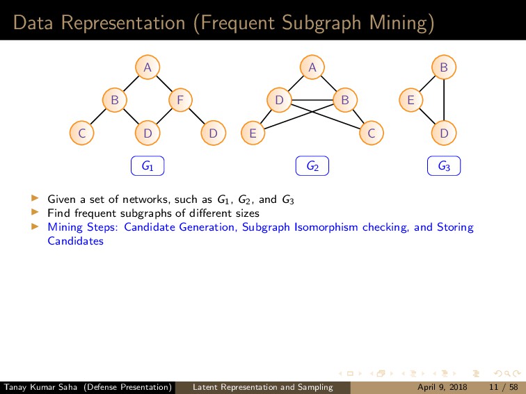
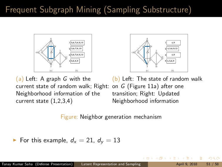
72. Frequent Subgraph Mining (Sampling Substructure) 1 2 3 4 5 7 6 9 8 10 11 12 (a) 1 5,6,7,8,9,10 2 5,6,7,8,10 3 5,6,7,8,9,10 4 5,6,8,9 (b) (a) Left: A graph G with the current state of random walk; Right: Neighborhood information of the current state (1,2,3,4) 1 2 3 4 5 7 6 9 8 10 11 12 (a) 1 4,9 2 4,5,6,9,12 3 4,9 8 4,5,6,9 (b) (b) Left: The state of random walk on G (Figure 11a) after one transition; Right: Updated Neighborhood information Figure: Neighbor generation mechanism For this example, dx = 21, dy = 13 Tanay Kumar Saha (Defense Presentation) Latent Representation and Sampling April 9, 2018 51 / 58
73. Frequent Subgraph Mining (Sampling Substructure) Algorithm 1: SampleIndSubGraph Pseudocode Input : - Graph Gi - Size of subgraph, [1]x ← State saved at Gi ; [2]dx ← Neighbor-count of x ; [3]a supx ← score of graph x ; [4]while a neighbor state y is not found do [5] y ← a random neighbor of x; [6] dy ← Neighbor count of y ; [7] a supy ← score of graph y ; [8] accp val ← (dx ∗ a supy )/(dy ∗ a supx ) ; [9] accp probablility ← min(1, accp val) ; [10] if uniform(0, 1) ≤ accp probability then [11] return y ; Tanay Kumar Saha (Defense Presentation) Latent Representation and Sampling April 9, 2018 52 / 58
74. Frequent Subgraph Mining (Sampling Substructure) Algorithm 2: SampleIndSubGraph Pseudocode Input : - Graph Gi - Size of subgraph, [1]x ← State saved at Gi ; [2]dx ← Neighbor-count of x ; [3]a supx ← score of graph x ; [4]while a neighbor state y is not found do [5] y ← a random neighbor of x; [6] dy ← Neighbor count of y ; [7] a supy ← score of graph y ; [8] accp val ← dx /dy ; [9] accp probablility ← min(1, accp val) ; [10] if uniform(0, 1) ≤ accp probability then [11] return y ; Tanay Kumar Saha (Defense Presentation) Latent Representation and Sampling April 9, 2018 53 / 58
75. Frequent Subgraph Mining (Sampling Substructure) The random walks are ergodic It satisfies reversibility condition, so, it achieves the target distribution We have use spectral gap (λ = 1 − max{λ1, |λm−1|}) technique to measure the mixing rate of our random walk We compute the mixing time (inverse of spectral gap) for size-6 subgraphs of Mutagen dataset and found that the mixing time is approximately around 15 units We suggest to use multiple chains along with a suitable distance measure (for example, jaccard distance) for choossing a suitable iteration count We show that the acceptance probability for our technique is quite high (a large number of rejected moves indicate a poorly designed proposal distribution) Table: Probability of Acceptance of FS3 for Mutagen and PS Dataset Mutagen PS = 8 =9 =10 =6 =7 Acceptance (%), Strat- egy =s1 82.70 ± 0.04 83.89 ± 0.03 81.66 ± 0.03 91.08 ± 0.01 92.23 ± 0.02 Acceptance (%), Strat- egy =s2 75.27 ± 0.05 76.74 ± 0.03 75.20 ± 0.03 85.08 ± 0.05 87.46 ± 0.06 Tanay Kumar Saha (Defense Presentation) Latent Representation and Sampling April 9, 2018 54 / 58
76. Functional Motif Detection Figure: Type 1 interface of TIM dimeric structure. (A) Loop 3 from subunit A and Loop 1 and Loop 4 from subunit B form a lock at the interface, and vice versa. (B) Surface view of Lock 1. (C) Residues of the loops involved in Lock 1 are shown in spheres. (D) Retrieved residues in Lock 1 are shown in bright color and others are deemed. Tanay Kumar Saha (Defense Presentation) Latent Representation and Sampling April 9, 2018 55 / 58
77. Outline 1 About Me 2 Thesis Contribution 3 Introduction and Motivation Data Representation 4 Our Approach for Modeling Temporal Smoothness in an Evolving Network Modeling Temporal Smoothness Solution Sketch Mathematical Formulation 5 Our Approach for Learning Sentence Representation Latent Representation of Sentences Description of Models Evaluation 6 Frequent Subgraph Mining Details of the Methods Some Results 7 Conclusion Tanay Kumar Saha (Defense Presentation) Latent Representation and Sampling April 9, 2018 56 / 58
78. Conclusion and Future Work Presented methods for capturing temporal smoothness Exploring non-linear deep models with large network Tanay Kumar Saha (Defense Presentation) Latent Representation and Sampling April 9, 2018 57 / 58
79. Conclusion and Future Work Presented methods for capturing temporal smoothness Exploring non-linear deep models with large network Novel models for learning vector representation of sentences that consider not only content of a sentence but also its context Two ways to incorporate context: retrofitting and regularizing Two types of context: discourse and similarity Discourse context beneficial for topic classification and clustering, whereas the similarity context beneficial for summarization Explore further how our models perform compared to existing compositional models, where documents with sentence-level sentiment annotation exists Tanay Kumar Saha (Defense Presentation) Latent Representation and Sampling April 9, 2018 57 / 58
80. Conclusion and Future Work Presented methods for capturing temporal smoothness Exploring non-linear deep models with large network Novel models for learning vector representation of sentences that consider not only content of a sentence but also its context Two ways to incorporate context: retrofitting and regularizing Two types of context: discourse and similarity Discourse context beneficial for topic classification and clustering, whereas the similarity context beneficial for summarization Explore further how our models perform compared to existing compositional models, where documents with sentence-level sentiment annotation exists Proposed sampling techniques for substructure mining Incorporating substructure information in the latent representation learning technique to infuse structural information Tanay Kumar Saha (Defense Presentation) Latent Representation and Sampling April 9, 2018 57 / 58
81. Thanks! Sen2Vec Code and Datasets: https://github.com/tksaha/con-s2v/tree/jointlearning Temporal node2vec Code: https://gitlab.com/tksaha/temporalnode2vec.git Motif Finding Code: https://github.com/tksaha/motif-finding Frequent Subgraph Mining Code: https://github.com/tksaha/fs3-graph-mining Finding Functional Motif Code: https://gitlab.com/tksaha/func motif Tanay Kumar Saha (Defense Presentation) Latent Representation and Sampling April 9, 2018 58 / 58