16/16
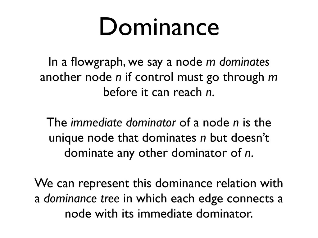
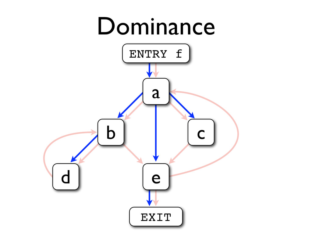
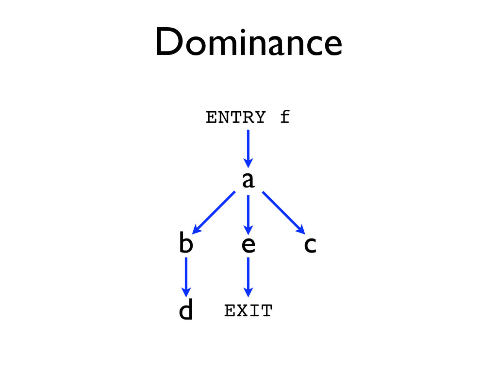
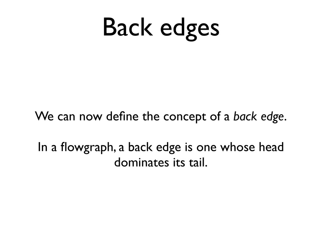
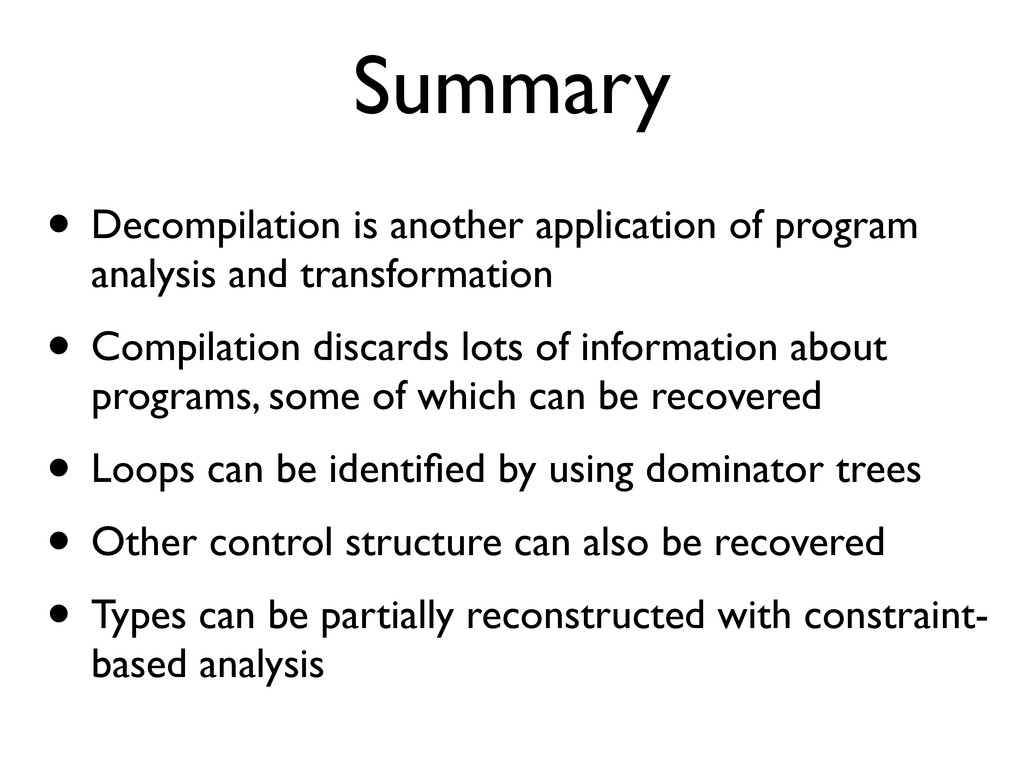
* Decompilation is another application of program analysis and transformation
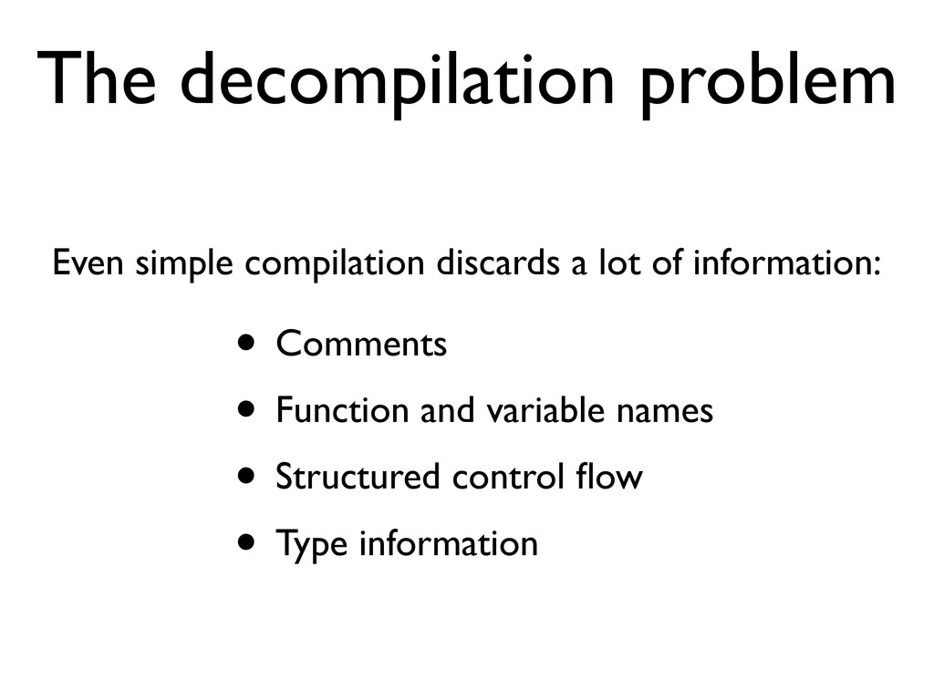
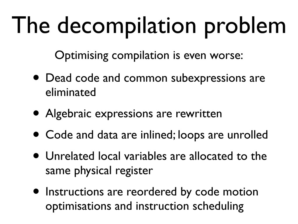
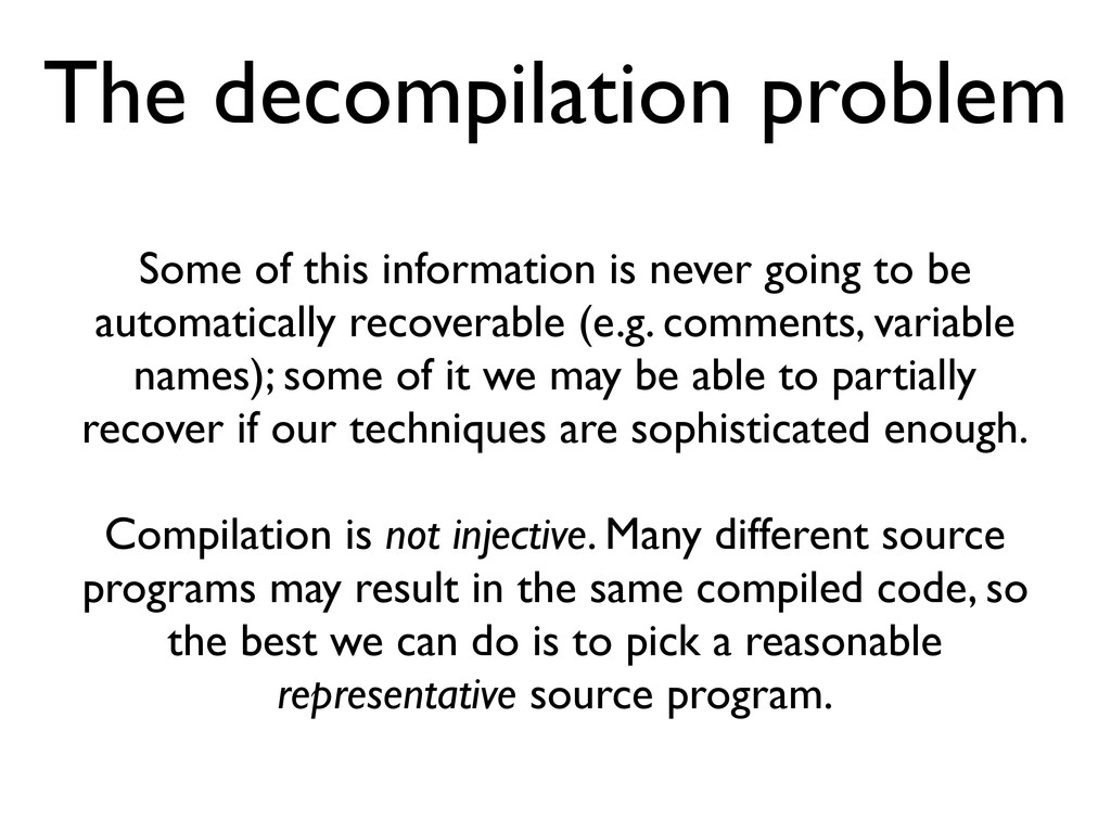
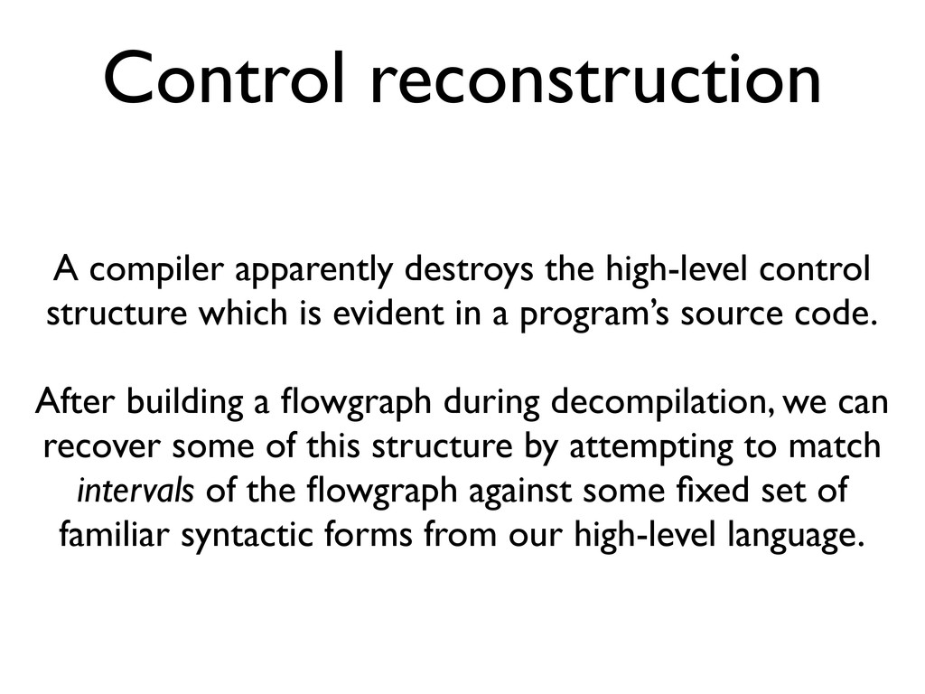
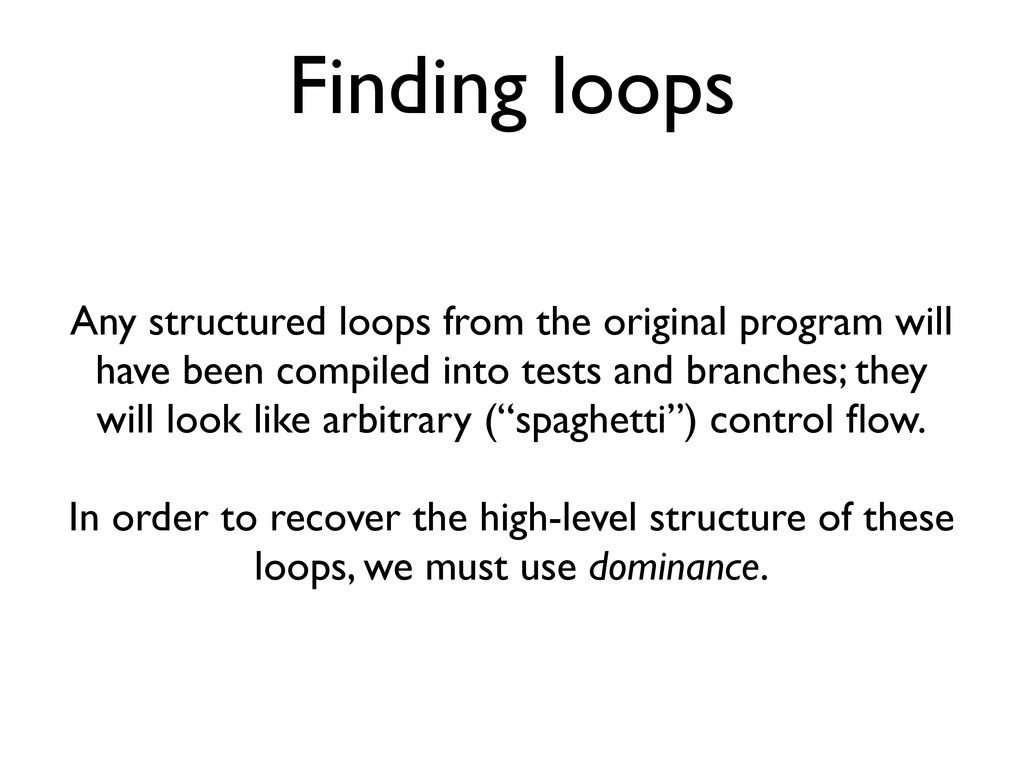
* Compilation discards lots of information about programs, some of which can be recovered
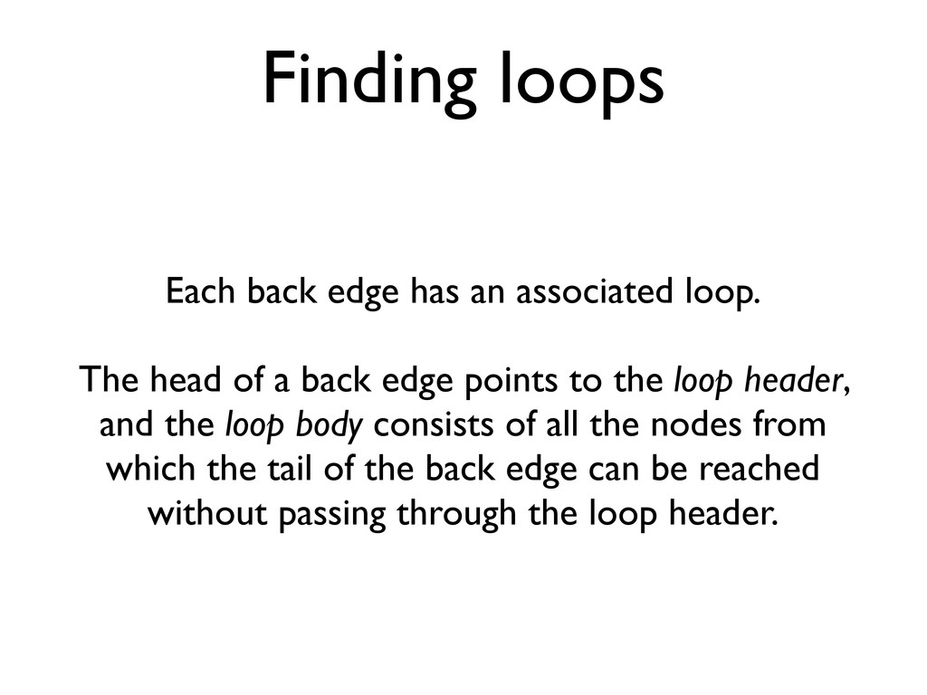
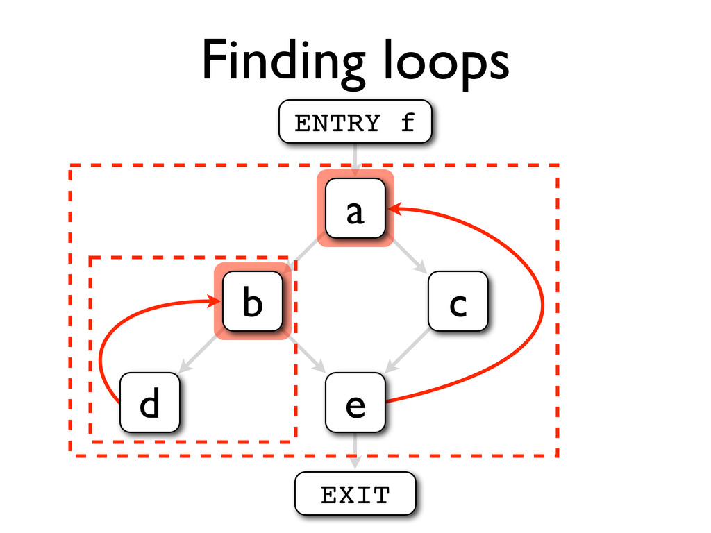
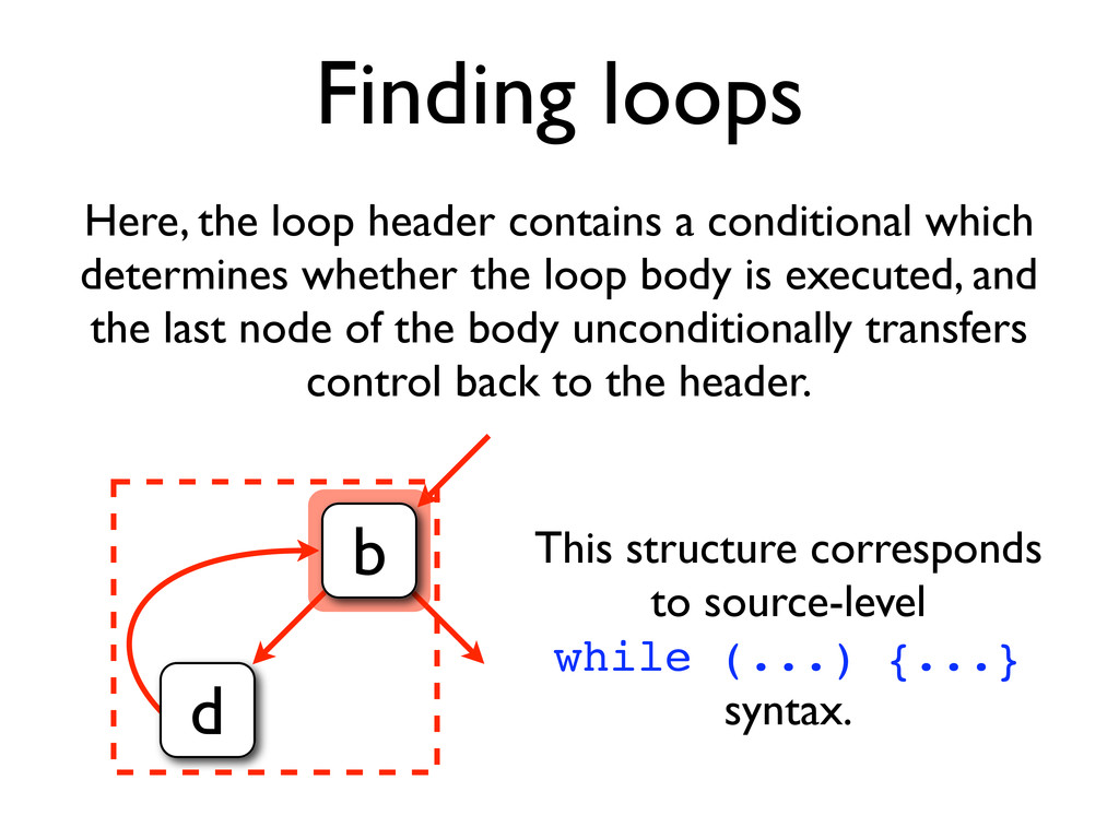
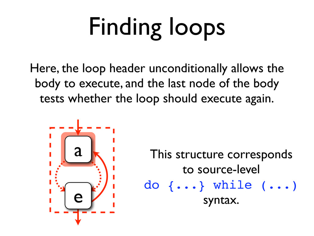
* Loops can be identified by using dominator trees
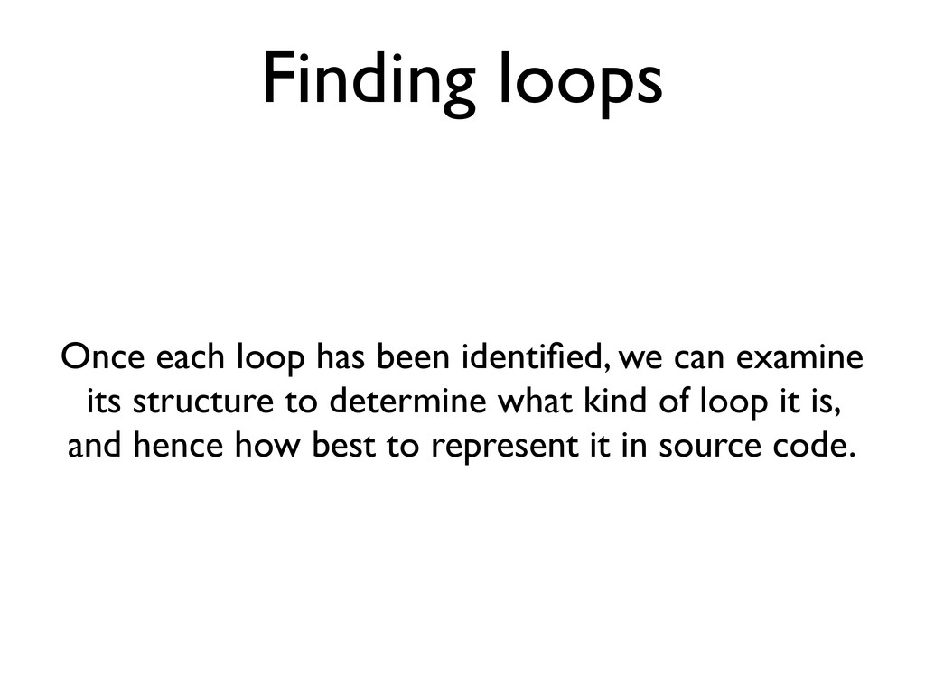
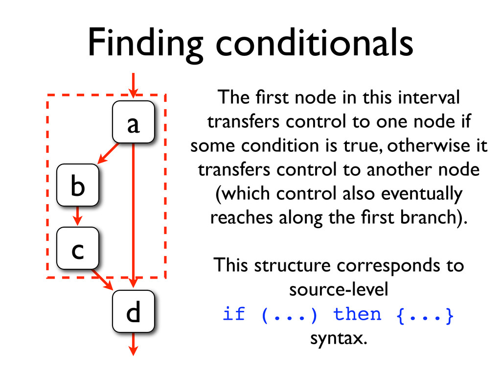
* Other control structure can also be recovered
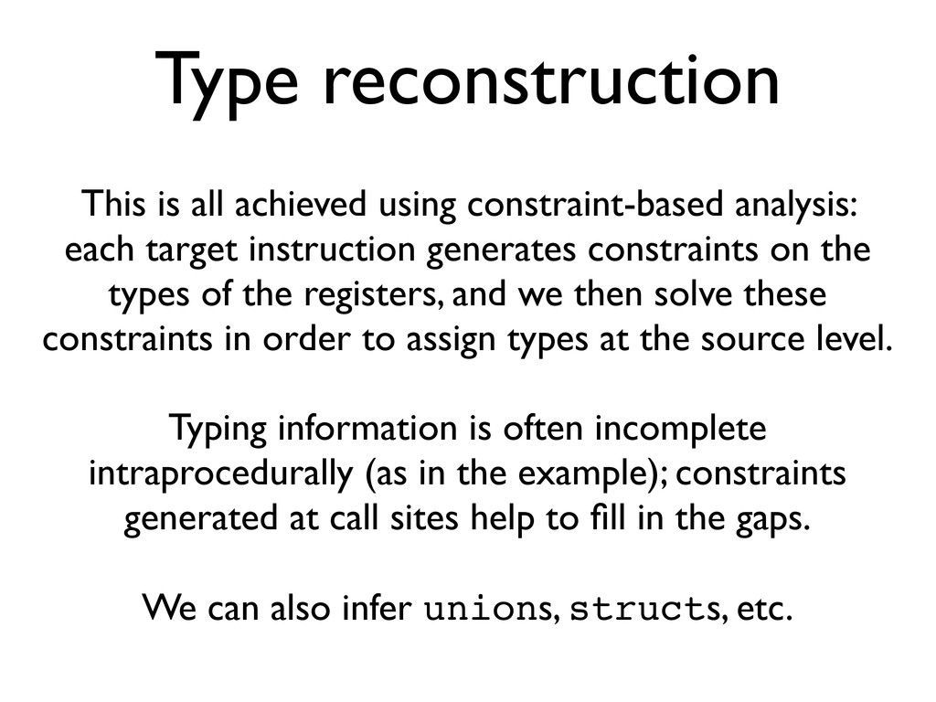
* Types can be partially reconstructed with constraint-based analysis
![Type reconstruction int foo (int *x) { return x[1] +](https://files.speakerdeck.com/presentations/4ea52505ca1be0005100a88e/slide_26.jpg)
![f: ldr r0,[r0,#4] add r0,r0,#2 mov r15,r14 ARM Type reconstruction](https://files.speakerdeck.com/presentations/4ea52505ca1be0005100a88e/slide_27.jpg)
![Type reconstruction int f (int *r0a) { return r0a[1] +](https://files.speakerdeck.com/presentations/4ea52505ca1be0005100a88e/slide_32.jpg)