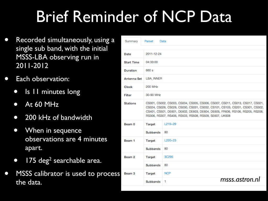
single sub band, with the initial MSSS-LBA observing run in 2011-2012 • Each observation: • Is 11 minutes long • At 60 MHz • 200 kHz of bandwidth • When in sequence observations are 4 minutes apart. • 175 deg2 searchable area. • MSSS calibrator is used to process the data. msss.astron.nl
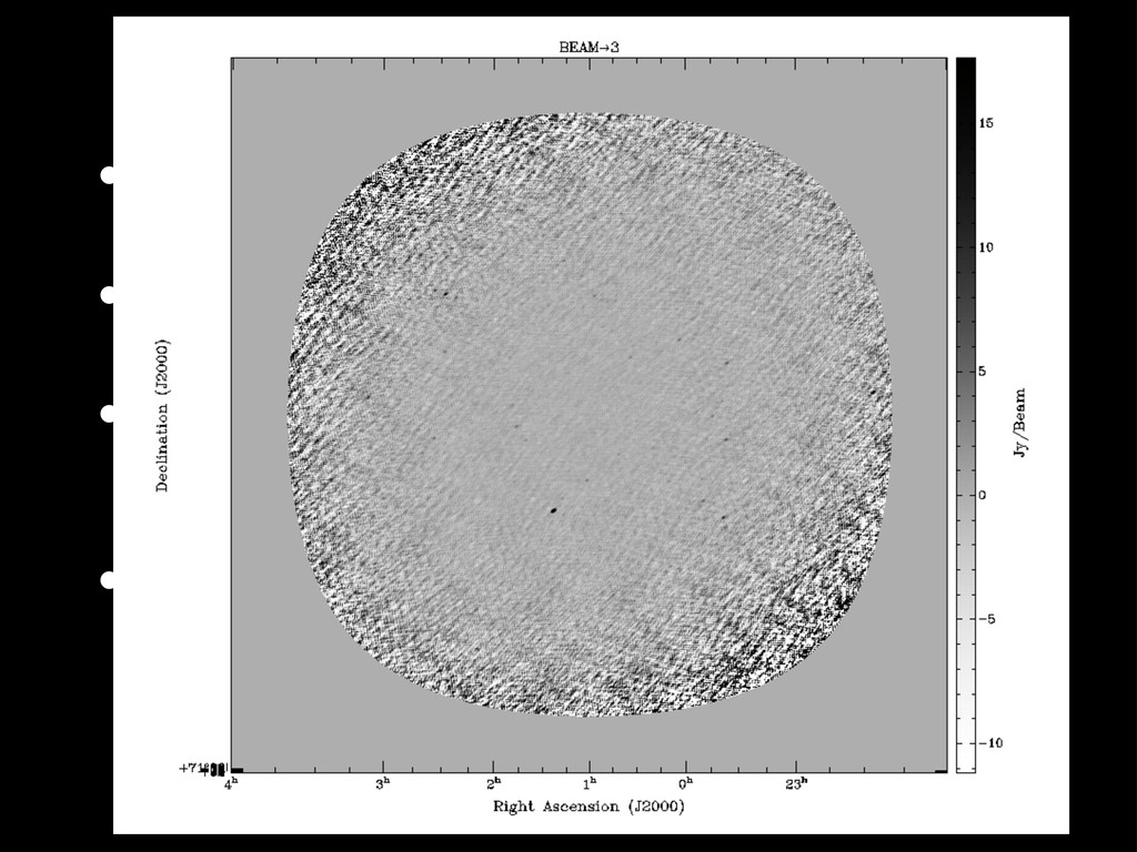
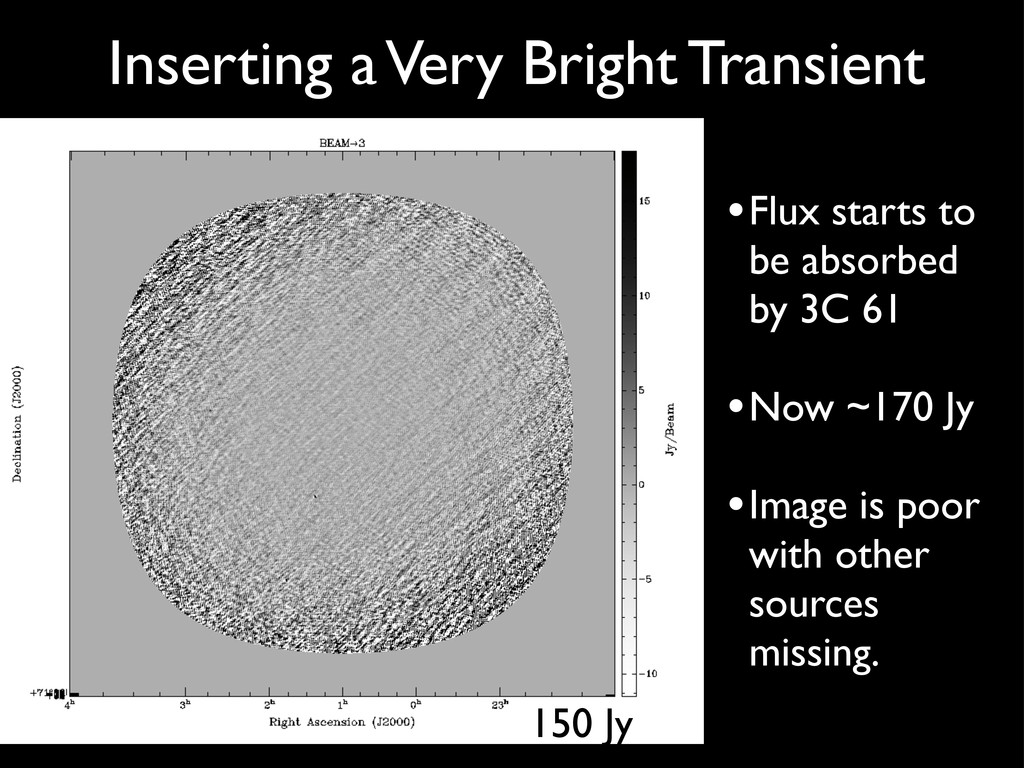
would react to a transient. • As we know, LOFAR reduction is quite dependent on the sky model used. • Nevertheless I wanted to confirm that a bright transient, not in the model, would appear or at least leave hints. • Eg. removing 3C 61.1 from the sky model, while causing bad artifacts, still leaves the source visible.
would react to a transient. • As we know, LOFAR reduction is quite dependent on the sky model used. • Nevertheless I wanted to confirm that a bright transient, not in the model, would appear or at least leave hints. • Eg. removing 3C 61.1 from the sky model, while causing bad artifacts, still leaves the source visible.
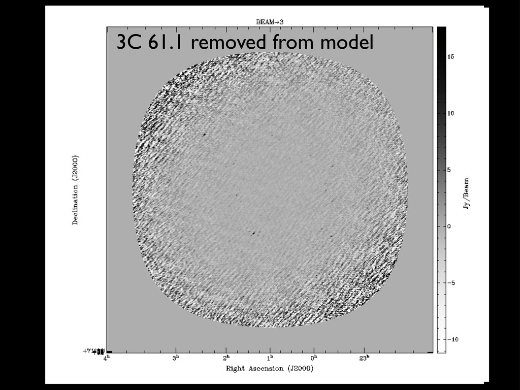
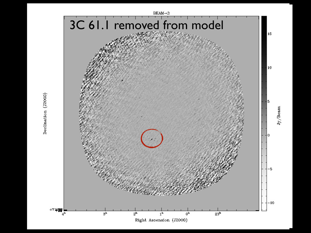
would react to a transient. • As we know, LOFAR reduction is quite dependent on the sky model used. • Nevertheless I wanted to confirm that a bright transient, not in the model, would appear or at least leave hints. • Eg. removing 3C 61.1 from the sky model, while causing bad artifacts, still leaves the source visible. 3C 61.1 removed from model
would react to a transient. • As we know, LOFAR reduction is quite dependent on the sky model used. • Nevertheless I wanted to confirm that a bright transient, not in the model, would appear or at least leave hints. • Eg. removing 3C 61.1 from the sky model, while causing bad artifacts, still leaves the source visible. 3C 61.1 removed from model
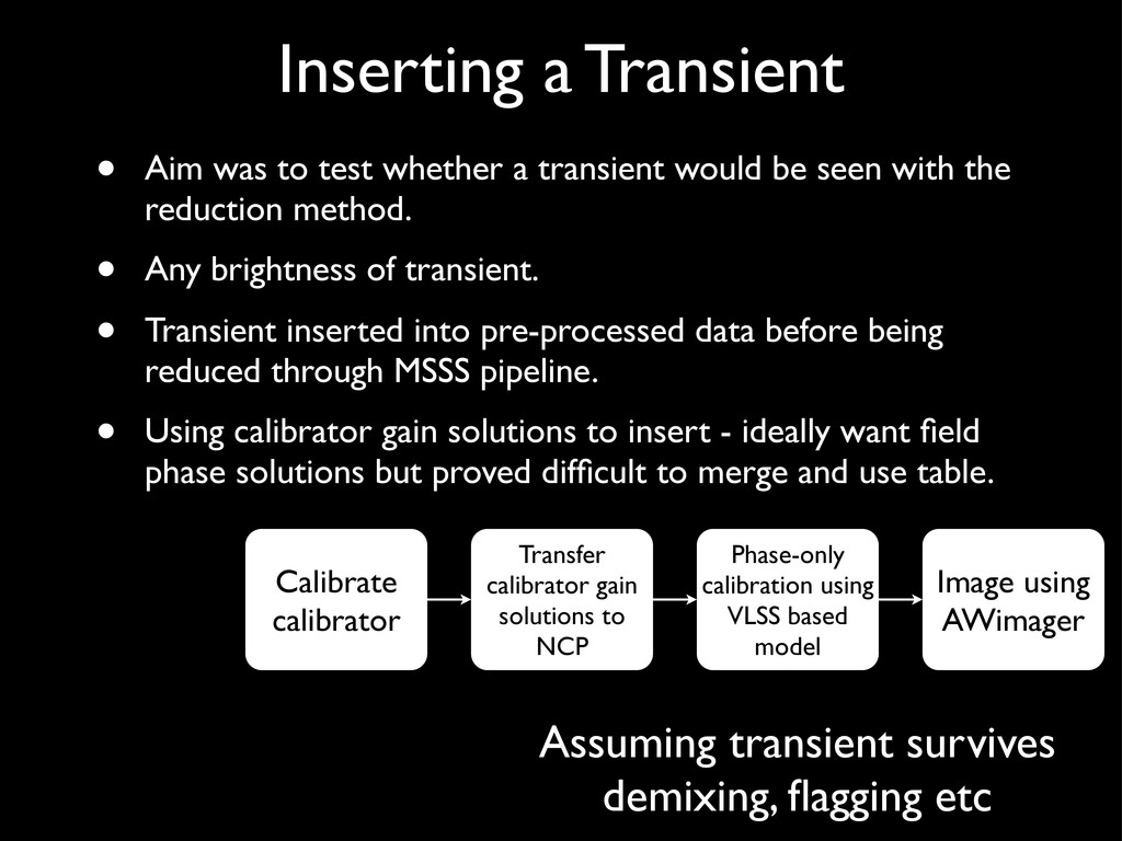
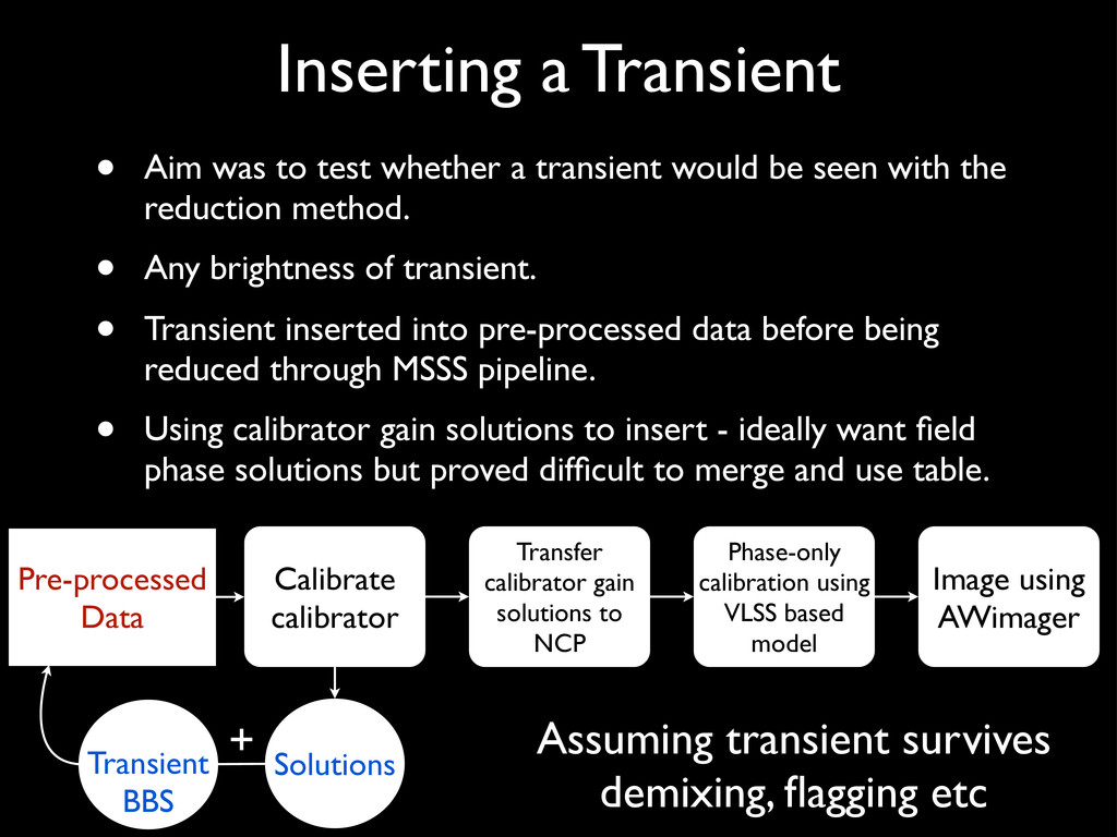
transient would be seen with the reduction method. • Any brightness of transient. • Transient inserted into pre-processed data before being reduced through MSSS pipeline. • Using calibrator gain solutions to insert - ideally want field phase solutions but proved difficult to merge and use table. Calibrate calibrator Transfer calibrator gain solutions to NCP Phase-only calibration using VLSS based model Image using AWimager Assuming transient survives demixing, flagging etc
transient would be seen with the reduction method. • Any brightness of transient. • Transient inserted into pre-processed data before being reduced through MSSS pipeline. • Using calibrator gain solutions to insert - ideally want field phase solutions but proved difficult to merge and use table. Calibrate calibrator Transfer calibrator gain solutions to NCP Phase-only calibration using VLSS based model Image using AWimager Pre-processed Data Solutions + Transient BBS Assuming transient survives demixing, flagging etc
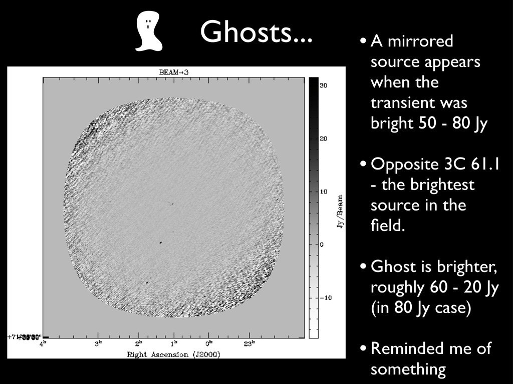
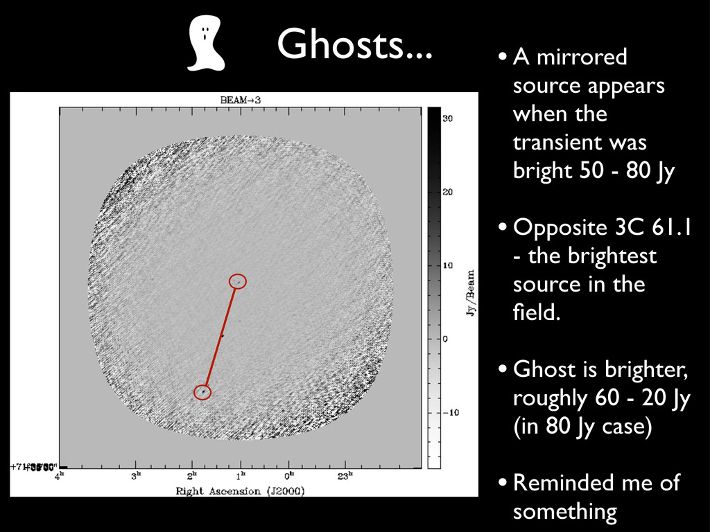
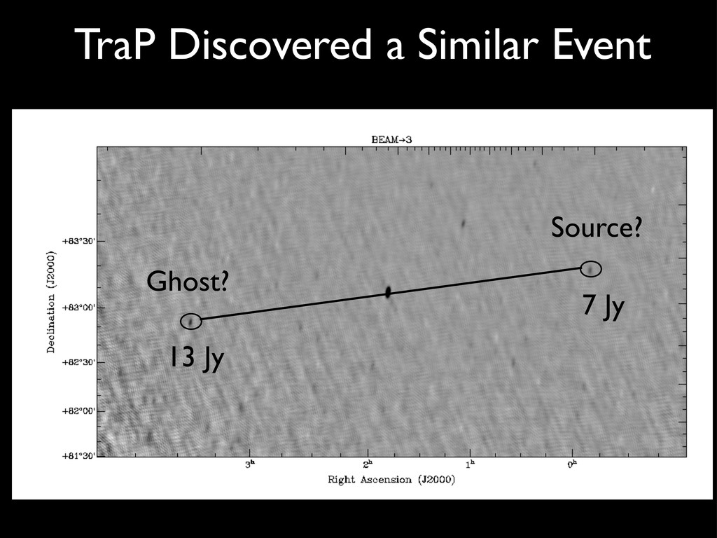
bright 50 - 80 Jy • Opposite 3C 61.1 - the brightest source in the field. • Ghost is brighter, roughly 60 - 20 Jy (in 80 Jy case) • Reminded me of something
bright 50 - 80 Jy • Opposite 3C 61.1 - the brightest source in the field. • Ghost is brighter, roughly 60 - 20 Jy (in 80 Jy case) • Reminded me of something
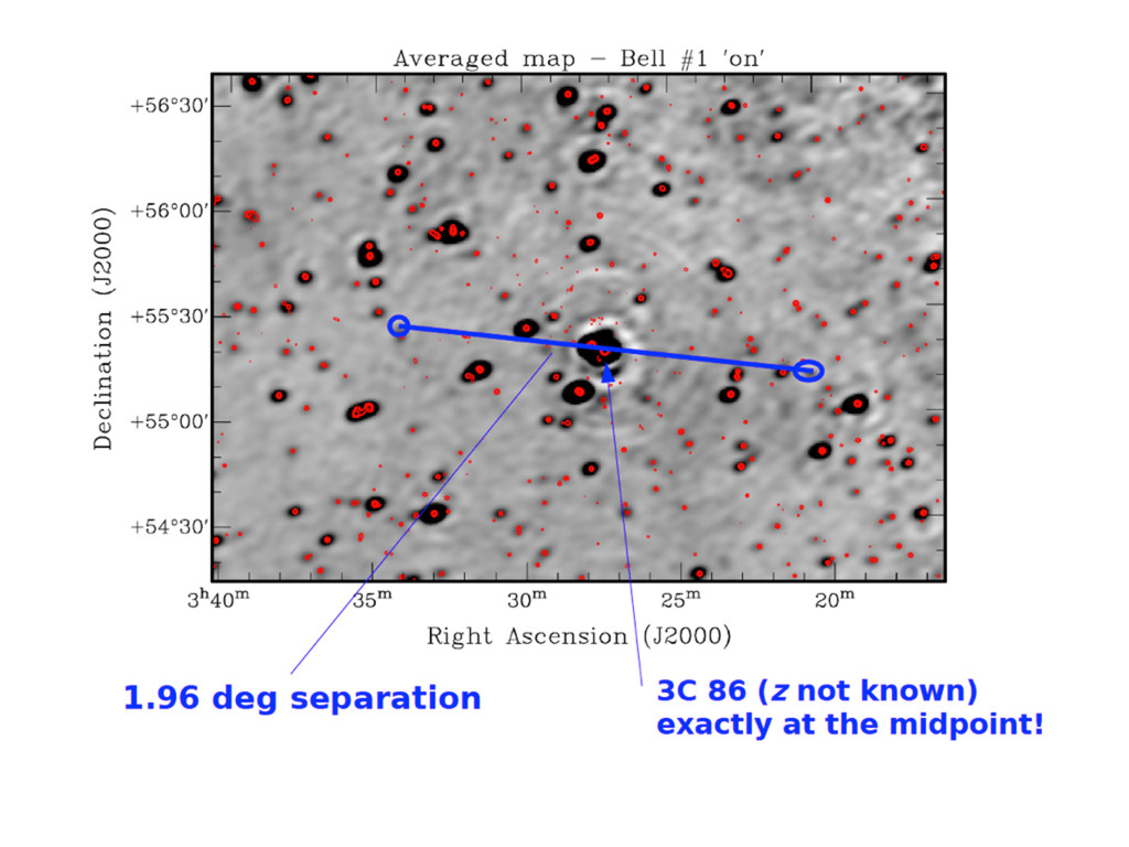
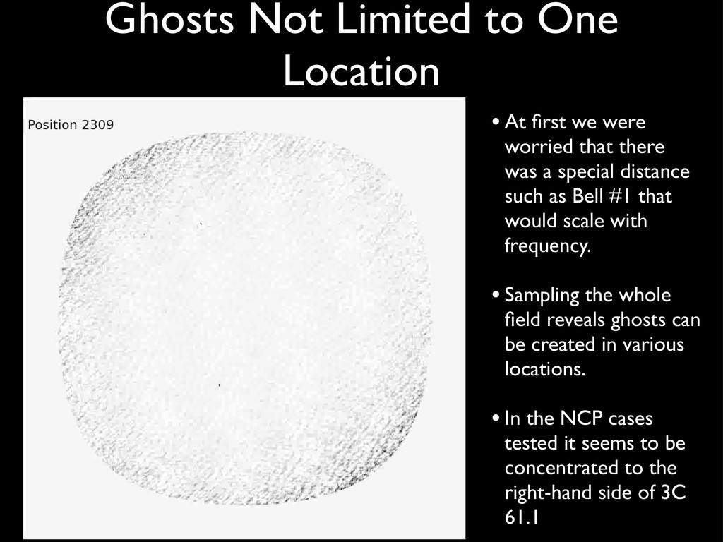
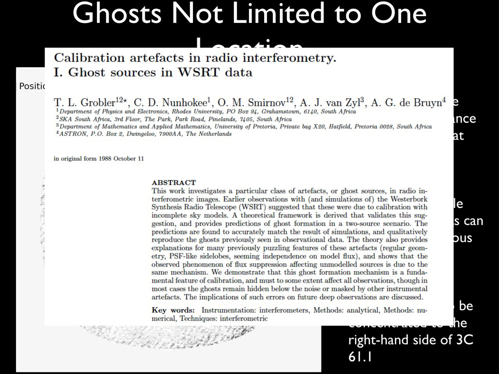
were worried that there was a special distance such as Bell #1 that would scale with frequency. • Sampling the whole field reveals ghosts can be created in various locations. • In the NCP cases tested it seems to be concentrated to the right-hand side of 3C 61.1
were worried that there was a special distance such as Bell #1 that would scale with frequency. • Sampling the whole field reveals ghosts can be created in various locations. • In the NCP cases tested it seems to be concentrated to the right-hand side of 3C 61.1
were worried that there was a special distance such as Bell #1 that would scale with frequency. • Sampling the whole field reveals ghosts can be created in various locations. • In the NCP cases tested it seems to be concentrated to the right-hand side of 3C 61.1
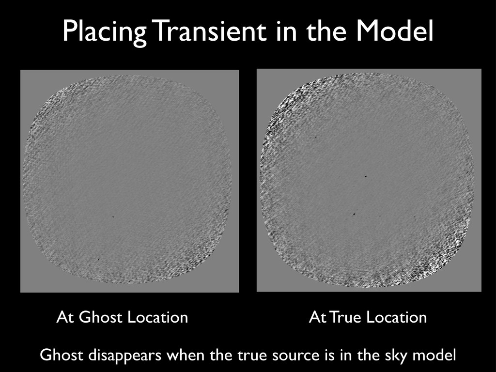
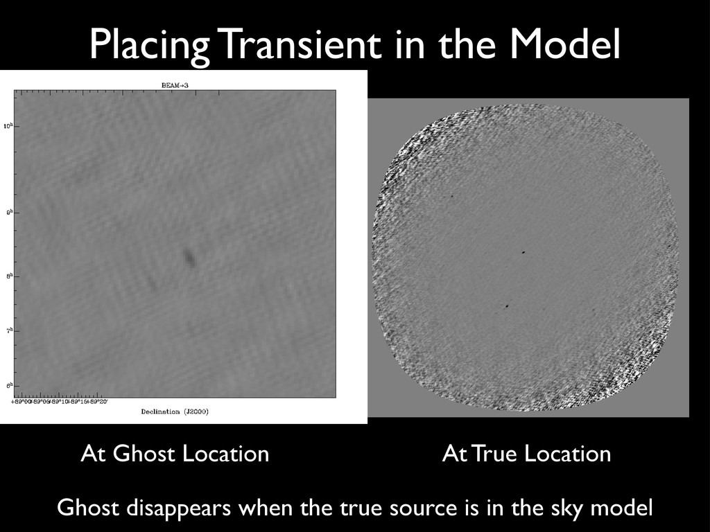
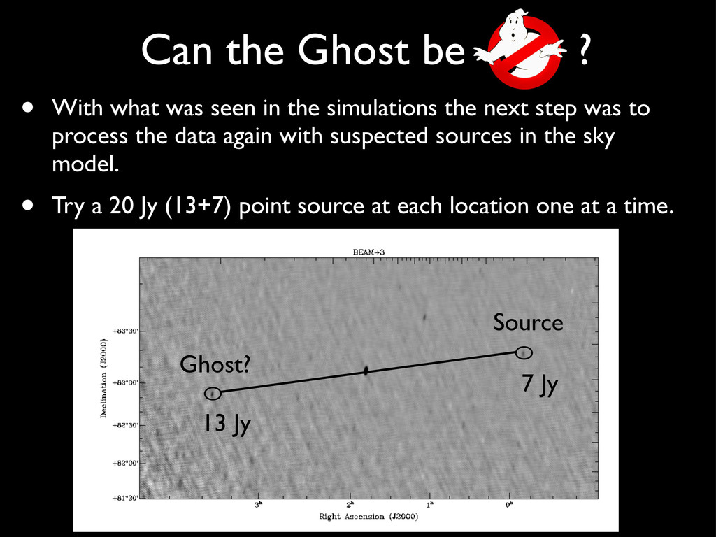
in the simulations the next step was to process the data again with suspected sources in the sky model. • Try a 20 Jy (13+7) point source at each location one at a time. 7 Jy Source Ghost? 13 Jy
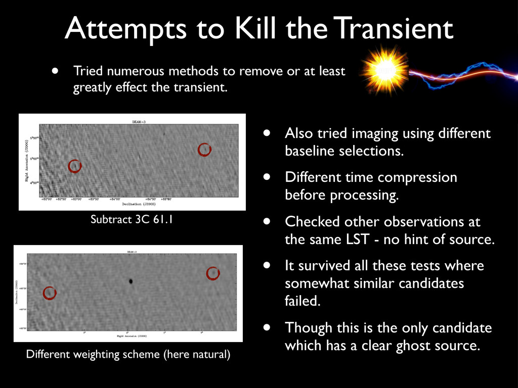
remove or at least greatly effect the transient. Subtract 3C 61.1 Different weighting scheme (here natural) • Also tried imaging using different baseline selections. • Different time compression before processing. • Checked other observations at the same LST - no hint of source. • It survived all these tests where somewhat similar candidates failed. • Though this is the only candidate which has a clear ghost source.
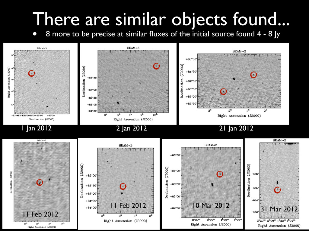
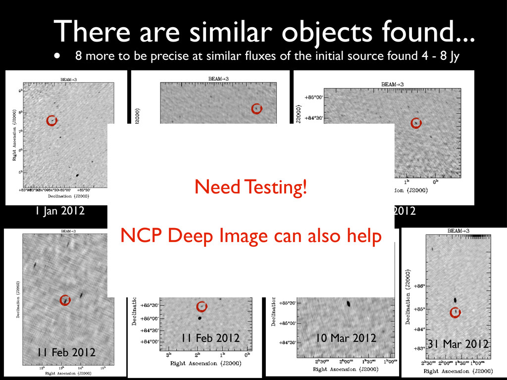
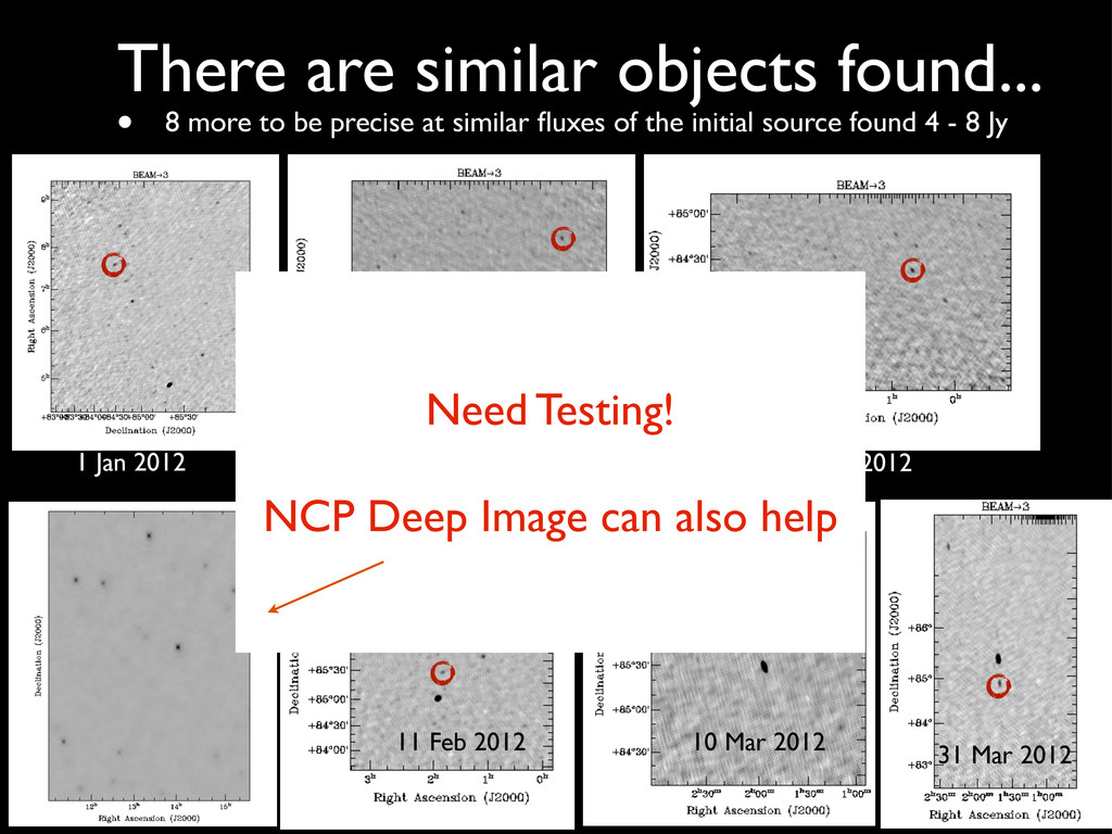
precise at similar fluxes of the initial source found 4 - 8 Jy 1 Jan 2012 2 Jan 2012 21 Jan 2012 11 Feb 2012 11 Feb 2012 10 Mar 2012 31 Mar 2012 Need Testing! NCP Deep Image can also help
precise at similar fluxes of the initial source found 4 - 8 Jy 1 Jan 2012 2 Jan 2012 21 Jan 2012 11 Feb 2012 11 Feb 2012 10 Mar 2012 31 Mar 2012 Need Testing! NCP Deep Image can also help
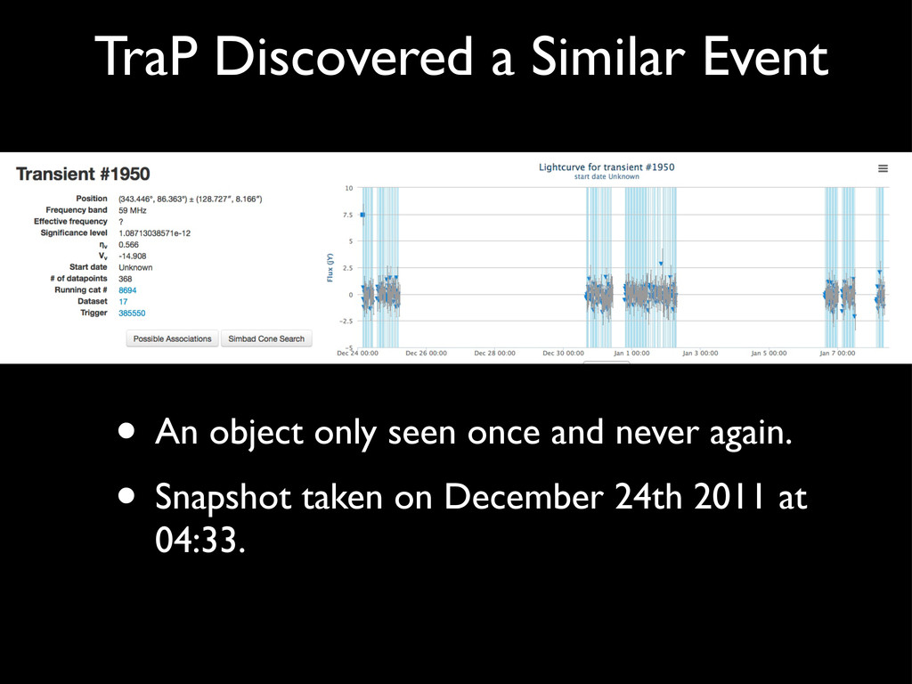
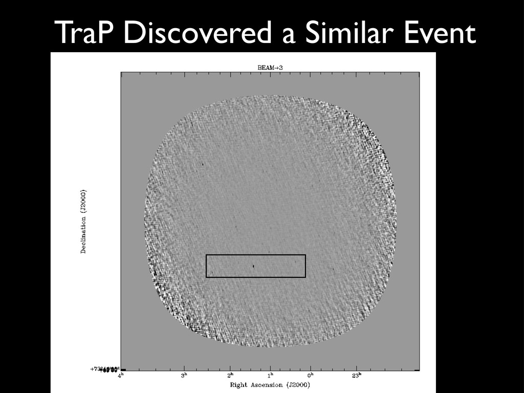
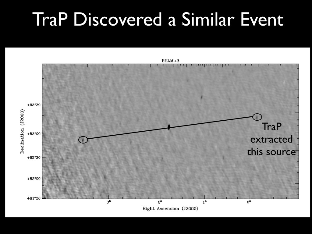
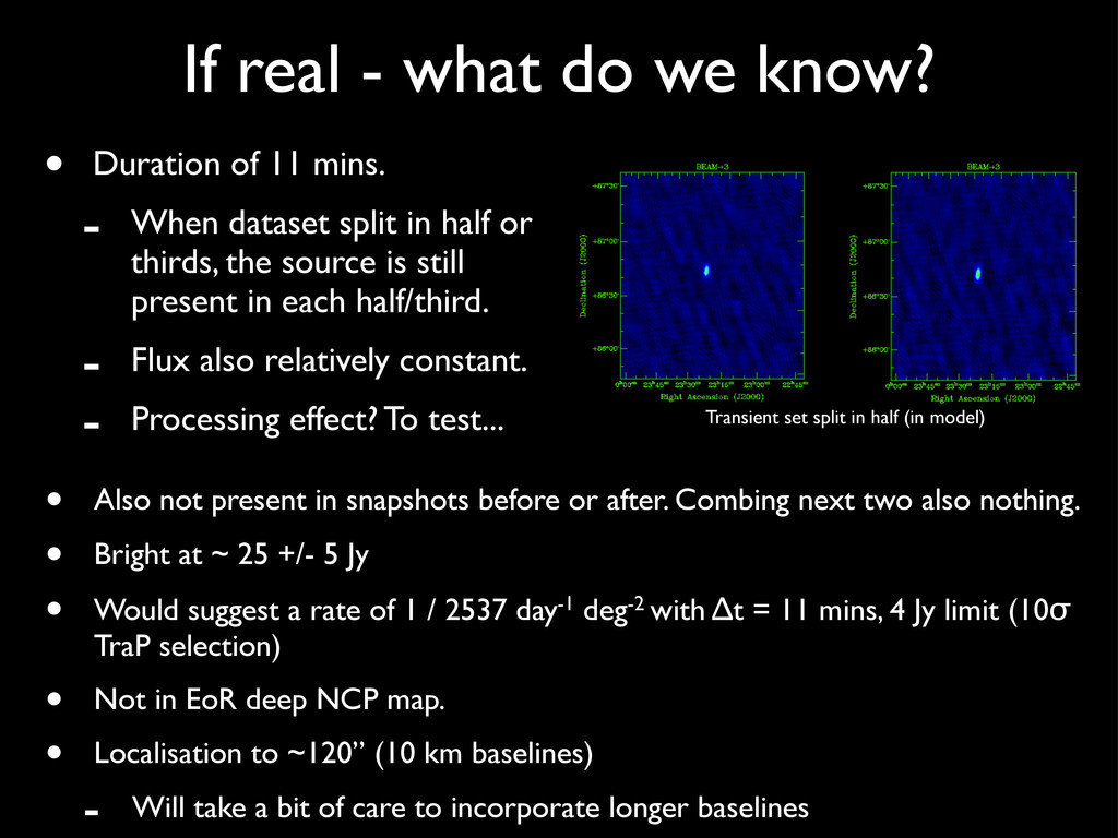
11 mins. - When dataset split in half or thirds, the source is still present in each half/third. - Flux also relatively constant. - Processing effect? To test... Transient set split in half (in model) • Also not present in snapshots before or after. Combing next two also nothing. • Bright at ~ 25 +/- 5 Jy • Would suggest a rate of 1 / 2537 day-1 deg-2 with ∆t = 11 mins, 4 Jy limit (10σ TraP selection) • Not in EoR deep NCP map. • Localisation to ~120” (10 km baselines) - Will take a bit of care to incorporate longer baselines
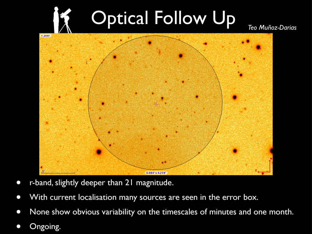
• With current localisation many sources are seen in the error box. • None show obvious variability on the timescales of minutes and one month. • Ongoing. Teo Muñoz-Darias
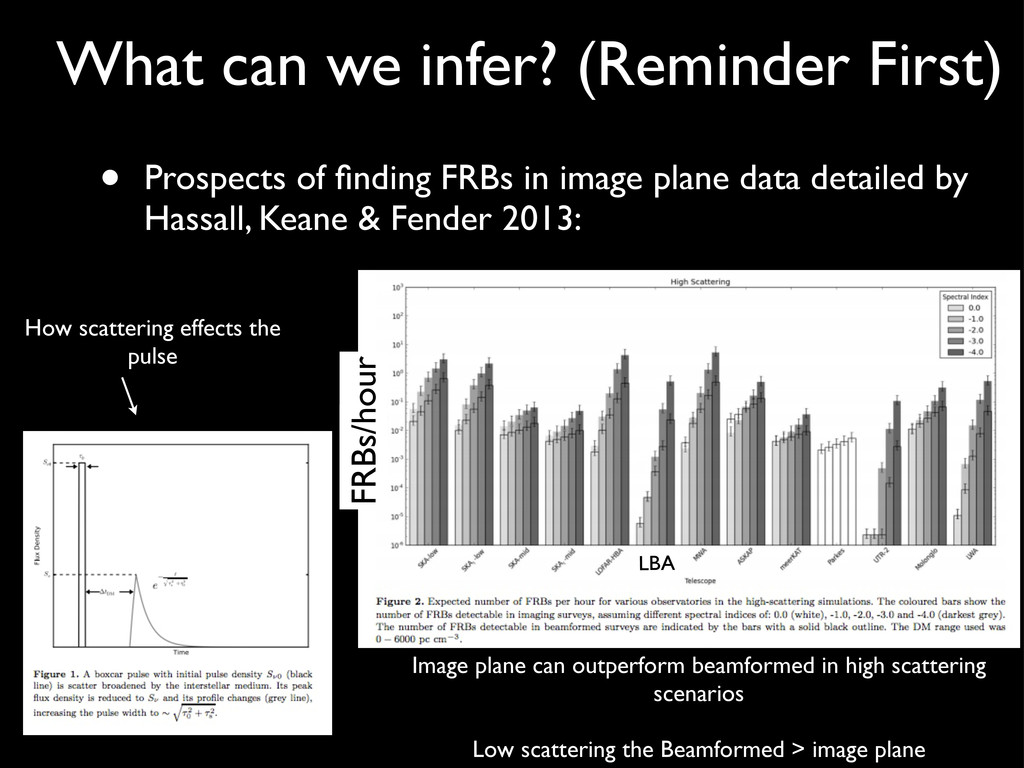
FRBs in image plane data detailed by Hassall, Keane & Fender 2013: How scattering effects the pulse Image plane can outperform beamformed in high scattering scenarios Low scattering the Beamformed > image plane FRBs/hour LBA
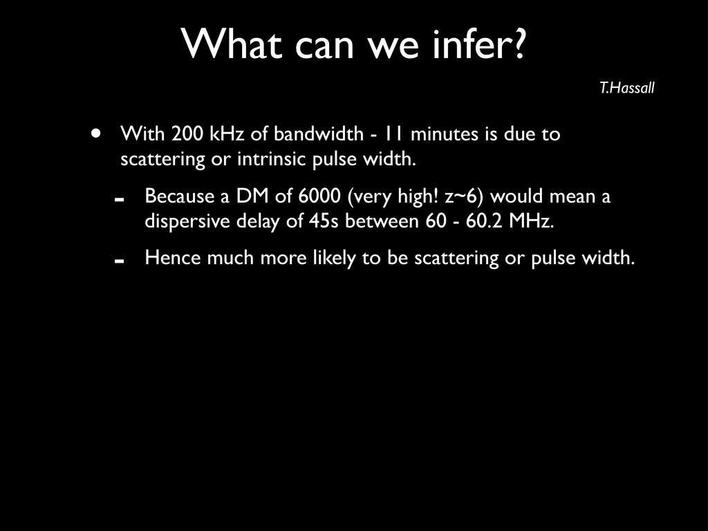
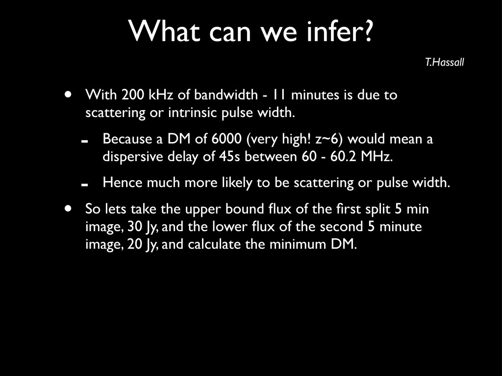
due to scattering or intrinsic pulse width. - Because a DM of 6000 (very high! z~6) would mean a dispersive delay of 45s between 60 - 60.2 MHz. - Hence much more likely to be scattering or pulse width. What can we infer? T.Hassall
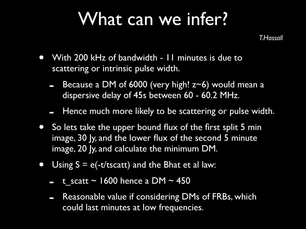
due to scattering or intrinsic pulse width. - Because a DM of 6000 (very high! z~6) would mean a dispersive delay of 45s between 60 - 60.2 MHz. - Hence much more likely to be scattering or pulse width. • So lets take the upper bound flux of the first split 5 min image, 30 Jy, and the lower flux of the second 5 minute image, 20 Jy, and calculate the minimum DM. What can we infer? T.Hassall
due to scattering or intrinsic pulse width. - Because a DM of 6000 (very high! z~6) would mean a dispersive delay of 45s between 60 - 60.2 MHz. - Hence much more likely to be scattering or pulse width. • So lets take the upper bound flux of the first split 5 min image, 30 Jy, and the lower flux of the second 5 minute image, 20 Jy, and calculate the minimum DM. • Using S = e(-t/tscatt) and the Bhat et al law: - t_scatt ~ 1600 hence a DM ~ 450 - Reasonable value if considering DMs of FRBs, which could last minutes at low frequencies. What can we infer? T.Hassall
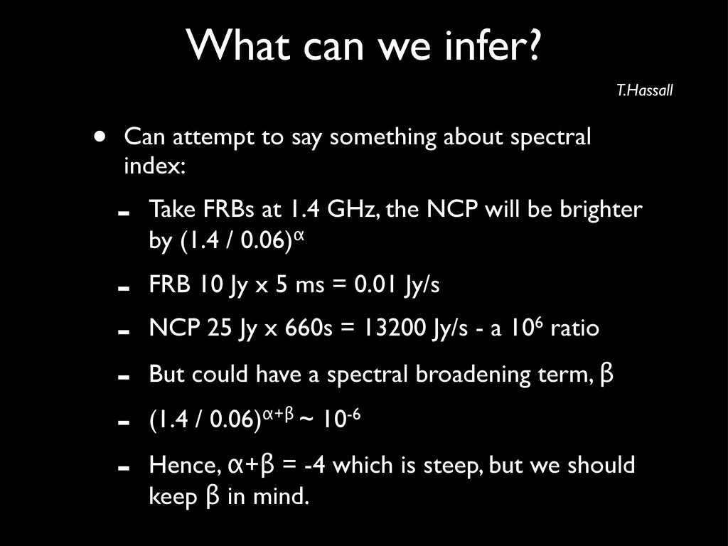
Take FRBs at 1.4 GHz, the NCP will be brighter by (1.4 / 0.06)α - FRB 10 Jy x 5 ms = 0.01 Jy/s - NCP 25 Jy x 660s = 13200 Jy/s - a 106 ratio - But could have a spectral broadening term, β - (1.4 / 0.06)α+β ~ 10-6 - Hence, α+β = -4 which is steep, but we should keep β in mind. What can we infer? T.Hassall
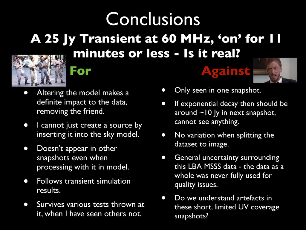
the data, removing the friend. • I cannot just create a source by inserting it into the sky model. • Doesn’t appear in other snapshots even when processing with it in model. • Follows transient simulation results. • Survives various tests thrown at it, when I have seen others not. For Against • Only seen in one snapshot. • If exponential decay then should be around ~10 Jy in next snapshot, cannot see anything. • No variation when splitting the dataset to image. • General uncertainty surrounding this LBA MSSS data - the data as a whole was never fully used for quality issues. • Do we understand artefacts in these short, limited UV coverage snapshots? A 25 Jy Transient at 60 MHz, ‘on’ for 11 minutes or less - Is it real?
blessing and a curse. • Perhaps will never be 100% sure because of this, but we have to take what we see. • Bell #1 situation of not being sure - Sky model tests on this data do not effect the transient. • Other candidates to check, may help in ways to prove/ disprove. • But this transient is tough to kill, it is yet to ever disappear. • RSM should be able to provide some answers...
Gijs, Bart and Tim et al • Previously data had been combined to gather decent images for humans to work with. • The TraP in it’s current state made searching these images possible.
function of time is: • S = exp(-t/t_scatt) • so 30/20 = exp(-660/t_scatt) • t_scatt = -660/ln(20/30) ~ 1600 • This corresponds to a DM~450 from the Bhat et al. law. Current DMs of FRBs are in the range 550-1100, so this seems very reasonable.