Sourcefinding Strategy in MSSS, the first LOFAR survey

Transcript

1. Sourcefinding strategy in MSSS, the first LOFAR survey DARIO CARBONE

   TKP meeting, 10 January 2014

2. Collaboration Job done in collaboration with: • the LOFAR Sourcefinder

   WG (led by Chiara Ferrari) http://www.lofar.org/operations/doku.php?id=commi • the MSSS team (led by George Heald) http://msss.astron.nl Dario Carbone

3. Outlines • PySE & PyBDSM – ASKAP Data Challenge –

   Performance – Parameters • MSSS – MVF – First catalog Dario Carbone

4. 4 Sourcefinder tools in LOFAR • Python Blob Detection and

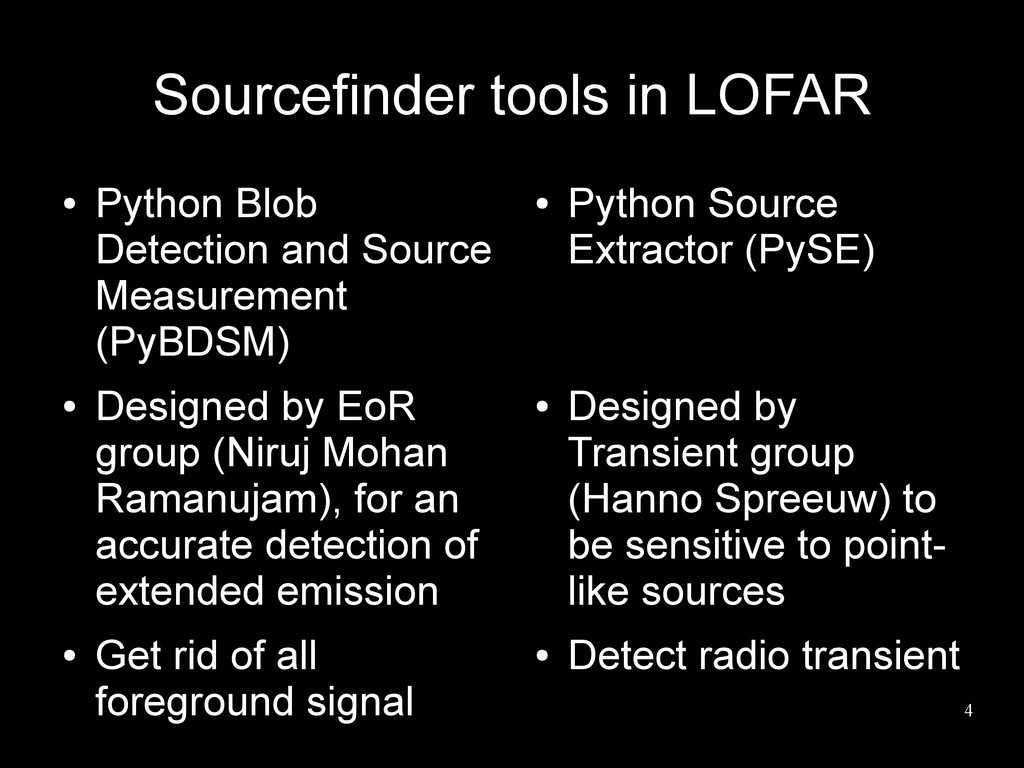
   Source Measurement (PyBDSM) • Designed by EoR group (Niruj Mohan Ramanujam), for an accurate detection of extended emission • Get rid of all foreground signal • Python Source Extractor (PySE) • Designed by Transient group (Hanno Spreeuw) to be sensitive to point- like sources • Detect radio transient

5. 5 PySE vs PyBDSM PySE is not able to detect

   extended sources Dario Carbone

6. 6 Focus on point-like sources • Radio transients are point-like

   sources • PySE was developed to find point-like sources • Speed requirements • Implemented in the TraP Dario Carbone

7. 7 PySE 1. Fit and subtract a variable background across

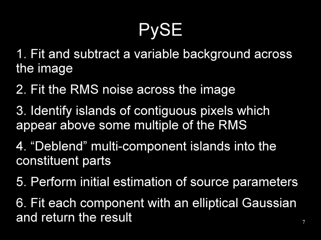
   the image 2. Fit the RMS noise across the image 3. Identify islands of contiguous pixels which appear above some multiple of the RMS 4. “Deblend” multi-component islands into the constituent parts 5. Perform initial estimation of source parameters 6. Fit each component with an elliptical Gaussian and return the result

8. 8 ASKAP Data Challenge Three simulated images including point sources

   and complex structures. 14 different sourcefinder tools participated.

9. 9 Challenge 2 – point sources only σRA σDec PySE

   0.39” 0.39” PyBDSM 0.44” 0.43” Credits to M. Whiting Dario Carbone

10. 10 Challenge 2 – PySE performance PySE completeness, reliability and

    flux recovery seems very good. • Force-beam option was turned on. Credits to M. Whiting Dario Carbone

11. 11 Challenge 3 – extended sources PySE isn't detecting extended

    sources, but isn't detecting fake ones. • Force-beam option was turned on. Credits to M. Whiting Dario Carbone

12. 12 Parameters for PySE Best parameters for source extraction with

    PySE: • grid size = 50 pixels • deblending turned on • deblending threshold = 90 • detection threshold = 8 σ • analysis threshold = 3 σ • Force-beam option turned on Dario Carbone

13. 13 Force-beam option • Avoid big ellipses collecting high flux

    • Only point-sources Dario Carbone

14. 14 The extracted flux can change just because the ellipse

    shape changed Flux Time Flux Time No force-beam With force-beam Force-beam option Dario Carbone

15. 15 • Very important for the transient pipeline • Source

    could not to be associated • Tests on 70 images of 10 fields, with a pixel size of 45 arcsec. Systematic position errors Dario Carbone

16. 16 Systematic position errors • • PyBDSM loses 13.3% PySE

    3.4% R DR = 5.68 Credits to A. Van der Horst Dario Carbone

17. 17 Systematic position errors • Systematic position error of 20

    arcsec • PyBDSM loses 2.0% PySE 1.0% Credits to A. Van der Horst R DR = 5.68 Dario Carbone

18. 18 MSSS intro • LBA: 30 − 75 MHz; 8x2

    MHz band • HBA: 119 − 158 MHz; 8x2 MHz band • Angular resolution ∼ 2′ • Sensitivity ∼ 10 mJy beam−1 http://msss.astron.nl Dario Carbone

19. 19 MSSS recap Heald et al., in prep. Dario Carbone

20. 20 MSSS Verification Field (MVF) • MSSS Verification Field (MVF):

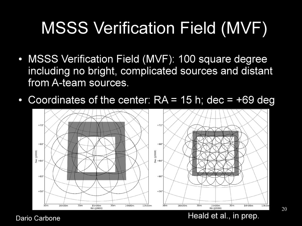
    100 square degree including no bright, complicated sources and distant from A-team sources. • Coordinates of the center: RA = 15 h; dec = +69 deg Heald et al., in prep. Dario Carbone

21. 21 MSSS Verification Field (MVF) LBA combined image of MVF

    Heald et al., in prep. HBA combined image of MVF Dario Carbone

22. 22 Source extraction strategy • Combined non-primary-beam-corrected image as detection

    image. • Run PyBDSM and PySE separately on each band and then combine the results. • For each sourcefinder, the detected sources are associated across the bands using the nearest neighbor criterion. • Catalogues from PyBDSM and PySE are then cross- matched. • Positions and fluxes are taken from PyBDSM outputs (if available). Dario Carbone

23. 23 Parameters for PySE • grid size = 50 pixels

    • deblending turned on • deblending threshold = 90 • detection threshold = 10 σ • analysis threshold = 5 σ • Force-beam option turned on Parameter settings based on real maps and simulations and the requirement to be conservative for this first catalogue. Dario Carbone

24. 24 Comparison • 697 sources are detected in the area

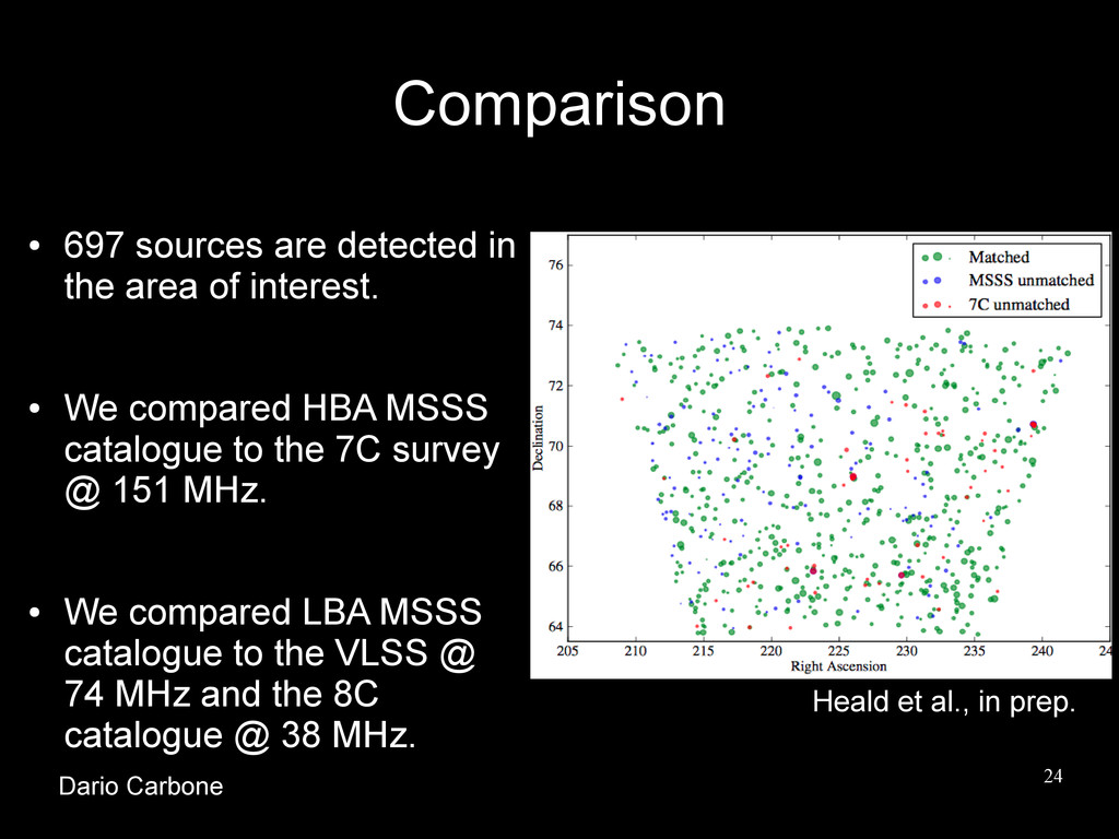
    of interest. • We compared HBA MSSS catalogue to the 7C survey @ 151 MHz. • We compared LBA MSSS catalogue to the VLSS @ 74 MHz and the 8C catalogue @ 38 MHz. Heald et al., in prep. Dario Carbone

25. 25 Column in MSSS catalogue • ID; Source ID, formed

    as Jhhmmss+ddmmss using the IAU convention. • RA & eRA; Source J2000 Right Ascension, in decimal degrees & error on Right Ascension, in seconds of time. • DEC & eDEC; Source J2000 Declination, in decimal degrees & error Declination, in arcseconds. • SFFLAG000; Flag indicating how many sourcefinders detected the source (0 means it was detected in both; 1 only in PyBDSM; 2 only in PYSE.) • Sint000 & eSint000; Source integrated flux at 000 MHz, in Jy & error on integrated flux, in Jy. • Spk000 & eSpk000; Source peak flux at 000 MHz, in Jy & error on peak flux, in Jy. • SLBA & eSLBA; LBA flux density (from combined map). Effective frequency is 000 MHz & error on LBA flux density. • SHBA & eSHBA; HBA flux density (from combined map). Effective frequency is 000 MHz & error on HBA flux density. • SPIX & eSPIX; Spectral index & error on spectral index. • SCURV & eSCURV; Spectral curvature & error on spectral curvature. • MAJAX000 & eMAJAX000; Major axis of fitted ellipse at 000 MHz & error on major axis. • MINAX000 & eMINAX000; Minor axis of fitted ellipse at 000 MHz & error on minor axis. • PA000 & ePA000; Position angle of fitted ellipse at 000 MHz, in degrees & error on position angle. Dario Carbone

26. 26 Column in MSSS catalogue • ID; Source ID, formed

    as Jhhmmss+ddmmss using the IAU convention. • RA & eRA; Source J2000 Right Ascension, in decimal degrees & error on Right Ascension, in seconds of time. • DEC & eDEC; Source J2000 Declination, in decimal degrees & error Declination, in arcseconds. • SFFLAG000; Flag indicating how many sourcefinders detected the source (0 means it was detected in both; 1 only in PyBDSM; 2 only in PYSE.) • Sint000 & eSint000; Source integrated flux at 000 MHz, in Jy & error on integrated flux, in Jy. • Spk000 & eSpk000; Source peak flux at 000 MHz, in Jy & error on peak flux, in Jy. • SLBA & eSLBA; LBA flux density (from combined map). Effective frequency is 000 MHz & error on LBA flux density. • SHBA & eSHBA; HBA flux density (from combined map). Effective frequency is 000 MHz & error on HBA flux density. • SPIX & eSPIX; Spectral index & error on spectral index. • SCURV & eSCURV; Spectral curvature & error on spectral curvature. • MAJAX000 & eMAJAX000; Major axis of fitted ellipse at 000 MHz & error on major axis. • MINAX000 & eMINAX000; Minor axis of fitted ellipse at 000 MHz & error on minor axis. • PA000 & ePA000; Position angle of fitted ellipse at 000 MHz, in degrees & error on position angle. This catalogue has 93 columns for the point sources, and 93 + 96 = 189 columns for extended sources!

27. 27 Conclusions • First catalogue of 100 squared degrees of

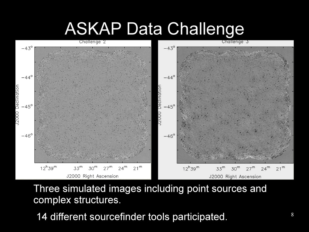
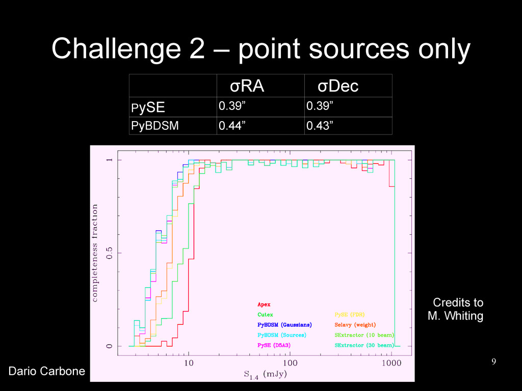
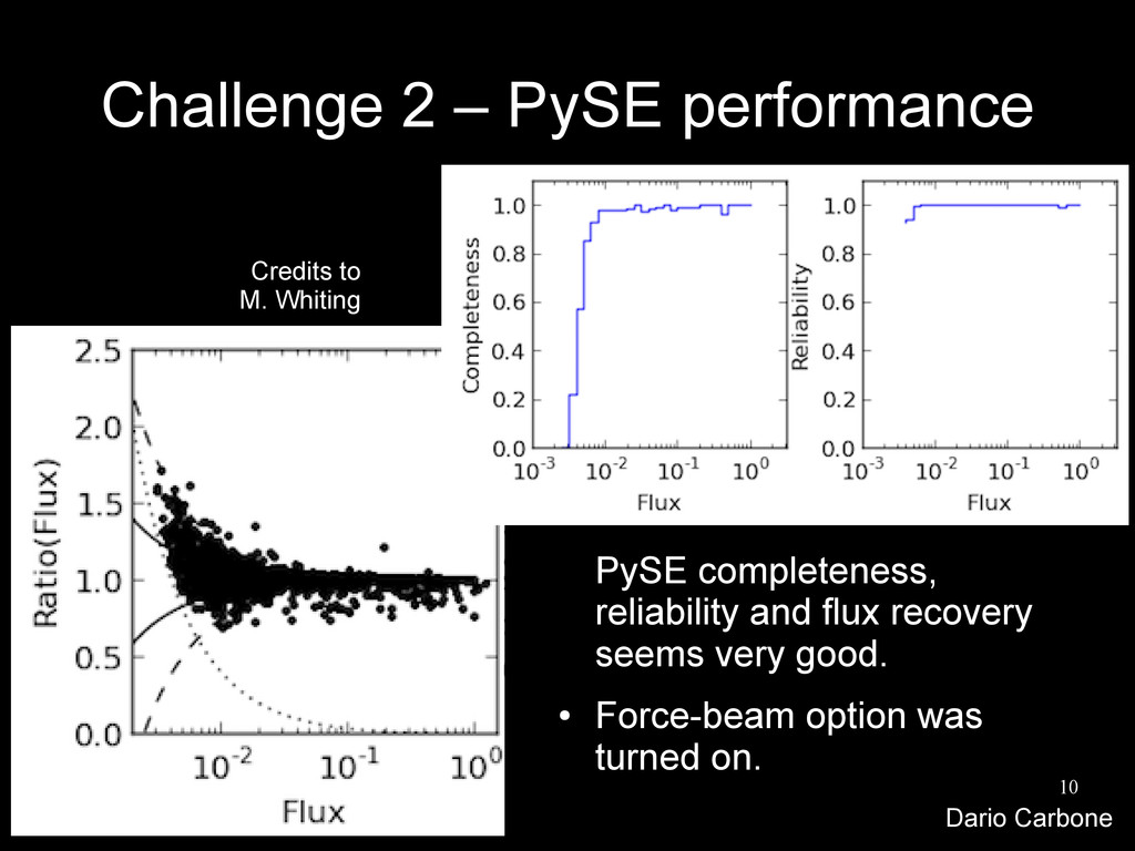
    MSSS is ready to be released. • This will contain a lot of data on several hundreds of sources. • Compared to other existing surveys at similar frequencies MSSS is behaving as expected. • Sourcefinding was done following a slightly more conservative approach than usual. • PySE is behaving very well on the Data Challenge maps as completeness, reliability, and flux recovery. • The force-beam option should be turned on as we are looking for point sources only.