Polarised Pulsars, the Ionosphere and LOFAR

Charlotte Sobey

Transcript

1. Intro ionFR LOFAR Summary I B0823+26 Summary II
   Polarised pulsars, the ionosphere, and LOFAR
   Charlotte Sobey
   csobey@mpifr-bonn.mpg.de
   Max-Planck-Institut f¨
   ur Radioastronomie
   5th Dec 2012
   Charlotte Sobey. MPIfR. TKP meeting Amsterdam. 05/12/12
   

   View Slide

2. Intro ionFR LOFAR Summary I B0823+26 Summary II
   Outline
   1 Calibration of High-Precision Faraday Rotation Measurements from
   LOFAR (A&A sub.)
   Motivation: why pulsar polarimetry and RMs?
   ionFR: introduction to model for ionospheric RM
   Comparisons: LOFAR observations vs. model
   2 Pulse modulation of PSR B0823+26
   Serendipity! surprising observation of pulsar switching ‘quiet’
   to ‘bright’ mode... emission mechanism
   Charlotte Sobey. MPIfR. TKP meeting Amsterdam. 05/12/12
   

   View Slide

3. Intro ionFR LOFAR Summary I B0823+26 Summary II
   Motivation
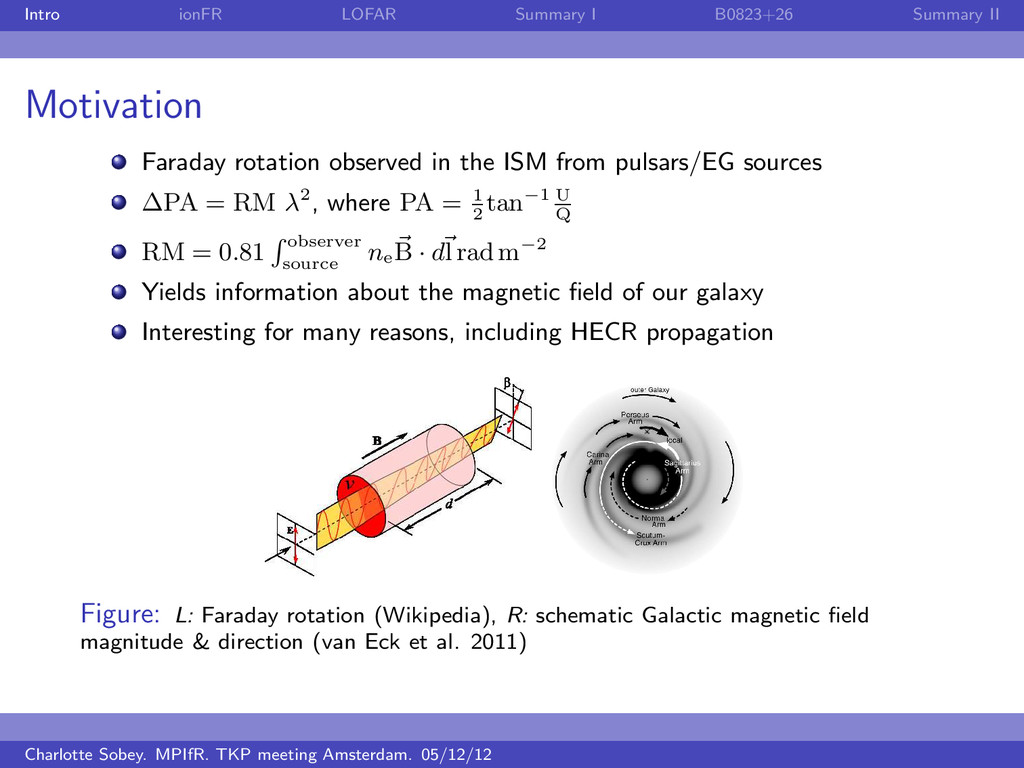
   Faraday rotation observed in the ISM from pulsars/EG sources
   ∆PA = RM λ2, where PA = 1
   2
   tan−1 U
   Q
   RM = 0.81 observer
   source
   ne
   B · dl rad m−2
   Yields information about the magnetic field of our galaxy
   Interesting for many reasons, including HECR propagation
   Figure: L: Faraday rotation (Wikipedia), R: schematic Galactic magnetic field
   magnitude & direction (van Eck et al. 2011)
   Charlotte Sobey. MPIfR. TKP meeting Amsterdam. 05/12/12
   

   View Slide

4. Intro ionFR LOFAR Summary I B0823+26 Summary II
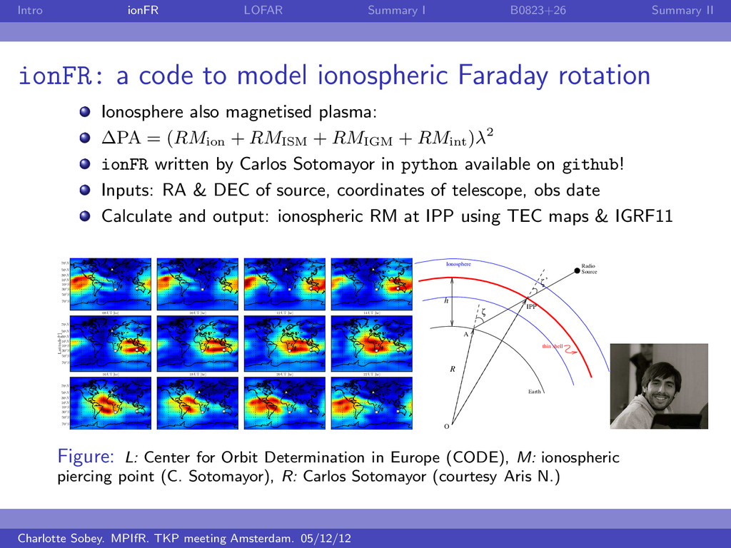
   ionFR: a code to model ionospheric Faraday rotation
   Ionosphere also magnetised plasma:
   ∆PA = (RMion
   + RMISM
   + RMIGM
   + RMint
   )λ2
   ionFR written by Carlos Sotomayor in python available on github!
   Inputs: RA & DEC of source, coordinates of telescope, obs date
   Calculate and output: ionospheric RM at IPP using TEC maps & IGRF11
   0.2
   0.4
   0.6
   0.8
   Latitude [◦]
   70◦S
   50◦S
   30◦S
   10◦S
   10◦N
   30◦N
   50◦N
   70◦N
   70◦S
   50◦S
   30◦S
   10◦S
   10◦N
   30◦N
   50◦N
   70◦N
   08 UT [hr] 10 UT [hr] 12 UT [hr] 14 UT [hr]
   70◦S
   50◦S
   30◦S
   10◦S
   10◦N
   30◦N
   50◦N
   70◦N
   16 UT [hr] 18 UT [hr] 20 UT [hr] 22 UT [hr]
   A
   IPP
   ζ
   ’
   O
   h
   R
   thin shell
   Ionosphere
   Earth
   Radio
   Source
   ζ
   Figure: L: Center for Orbit Determination in Europe (CODE), M: ionospheric
   piercing point (C. Sotomayor), R: Carlos Sotomayor (courtesy Aris N.)
   Charlotte Sobey. MPIfR. TKP meeting Amsterdam. 05/12/12
   

   View Slide

5. Intro ionFR LOFAR Summary I B0823+26 Summary II
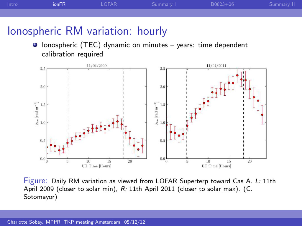
   Ionospheric RM variation: hourly
   Ionospheric (TEC) dynamic on minutes – years: time dependent
   calibration required
   Figure: Daily RM variation as viewed from LOFAR Superterp toward Cas A. L: 11th
   April 2009 (closer to solar min), R: 11th April 2011 (closer to solar max). (C.
   Sotomayor)
   Charlotte Sobey. MPIfR. TKP meeting Amsterdam. 05/12/12
   

   View Slide

6. Intro ionFR LOFAR Summary I B0823+26 Summary II
   Ionospheric RM variation: yearly
   Ionospheric (TEC) dynamic on minutes – years: time dependent
   calibration required
   Essential for monitoring RMs in the ISM over several epochs
   Apr 98 Mar 00 Feb 02 Jan 04 Dec 05 Nov 07 Oct 09 Sep 11
   0
   2
   4
   6
   8
   10
   |φion
   | [rad m−2]
   Apr 98 Mar 00 Feb 02 Jan 04 Dec 05 Nov 07 Oct 09 Sep 11
   0
   5
   10
   15
   20
   25
   |φion
   | [rad m−2]
   Figure: Weekly averages of the maximum and minimum (blue and red lines, respectively) absolute ionospheric
   Faraday depth. L: towards CasA viewed from LOFAR, R: towards Eta Carinae viewed from average of SKA core
   sites in Western Australia and South Africa. (C. Sotomayor)
   Charlotte Sobey. MPIfR. TKP meeting Amsterdam. 05/12/12
   

   View Slide

7. Intro ionFR LOFAR Summary I B0823+26 Summary II
   RM-synthesis
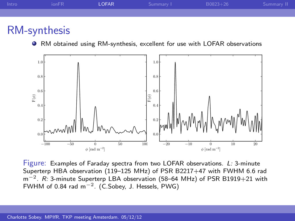
   RM obtained using RM-synthesis, excellent for use with LOFAR observations
   −100 −50 0 50 100
   φ [rad m−2]
   0.0
   0.2
   0.4
   0.6
   0.8
   1.0
   F(φ)
   −20 −10 0 10 20
   φ [rad m−2]
   0.0
   0.2
   0.4
   0.6
   0.8
   1.0
   F(φ)
   Figure: Examples of Faraday spectra from two LOFAR observations. L: 3-minute
   Superterp HBA observation (119–125 MHz) of PSR B2217+47 with FWHM 6.6 rad
   m−2. R: 3-minute Superterp LBA observation (58–64 MHz) of PSR B1919+21 with
   FWHM of 0.84 rad m−2. (C.Sobey, J. Hessels, PWG)
   Charlotte Sobey. MPIfR. TKP meeting Amsterdam. 05/12/12
   

   View Slide

8. Intro ionFR LOFAR Summary I B0823+26 Summary II
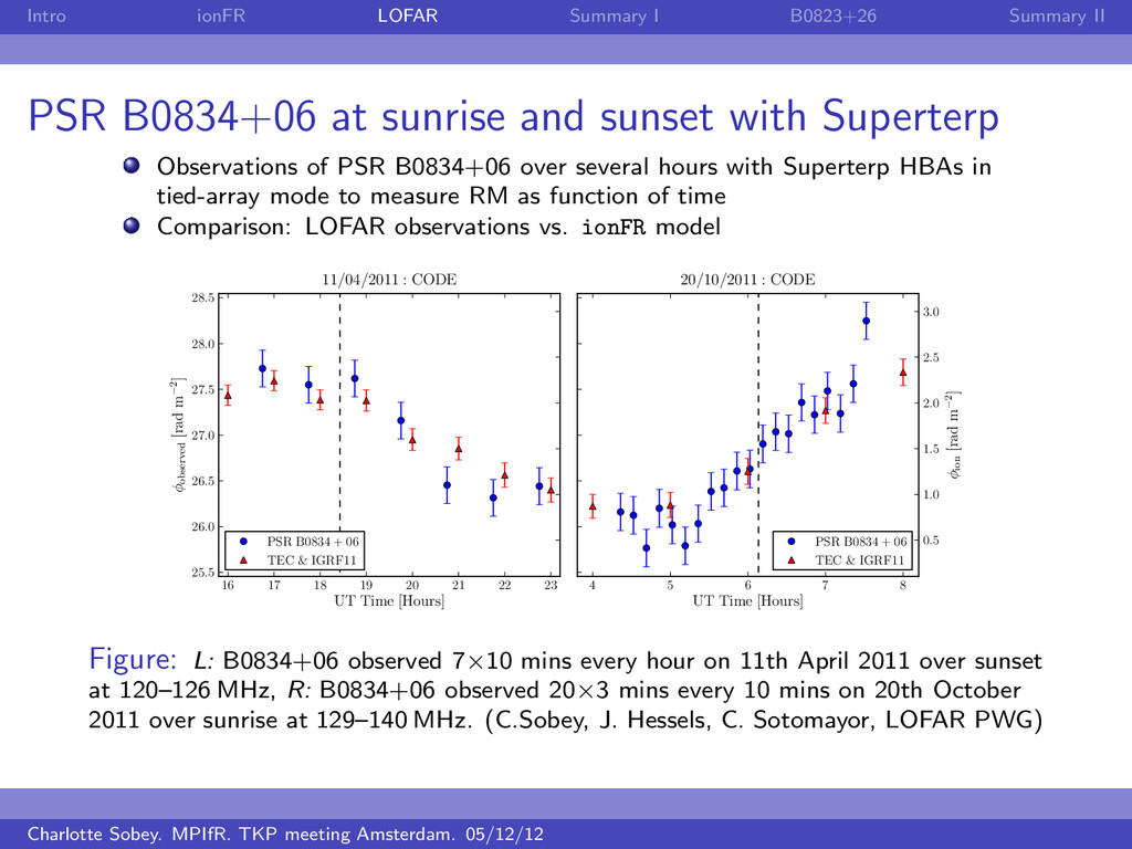
   PSR B0834+06 at sunrise and sunset with Superterp
   Observations of PSR B0834+06 over several hours with Superterp HBAs in
   tied-array mode to measure RM as function of time
   Comparison: LOFAR observations vs. ionFR model
   16 17 18 19 20 21 22 23
   UT Time [Hours]
   25.5
   26.0
   26.5
   27.0
   27.5
   28.0
   28.5
   φobserved
   [rad m−2]
   11/04/2011 : CODE
   PSR B0834 + 06
   TEC & IGRF11
   4 5 6 7 8
   UT Time [Hours]
   20/10/2011 : CODE
   0.5
   1.0
   1.5
   2.0
   2.5
   3.0
   φion
   [rad m−2]
   PSR B0834 + 06
   TEC & IGRF11
   Figure: L: B0834+06 observed 7×10 mins every hour on 11th April 2011 over sunset
   at 120–126 MHz, R: B0834+06 observed 20×3 mins every 10 mins on 20th October
   2011 over sunrise at 129–140 MHz. (C.Sobey, J. Hessels, C. Sotomayor, LOFAR PWG)
   Charlotte Sobey. MPIfR. TKP meeting Amsterdam. 05/12/12
   

   View Slide

9. Intro ionFR LOFAR Summary I B0823+26 Summary II
   Comparison of TEC data sources
   Many research groups provide ionospheric TEC maps
   Resolution and time cadence varies
   CODE: global maps with 2 hour, 5×2.5◦ resolution, via ftp download (left)
   ROB: European maps with 15 minute, 0.5×0.5◦ resolution, via email
   (right)LOFAR
   40◦N
   50◦N
   60◦N
   19.5◦W 9.5◦W 0.5◦E 10.5◦E 20.5◦E
   VTEC map (0.5◦ × 0.5◦grid) − 2012/03/23/00 : 00 : 00 UT
   4.5
   6.0
   7.5
   9.0
   10.5
   12.0
   13.5
   15.0
   TECU
   Figure: L: CODE, R: ROB (C. Sotomayor)
   Charlotte Sobey. MPIfR. TKP meeting Amsterdam. 05/12/12
   

   View Slide

10. Intro ionFR LOFAR Summary I B0823+26 Summary II
    Three PSRs at sunrise with Superterp
    Observations of PSRs B1642−03, B1919+21, B2217+47 with Superterp
    HBAs/LBAs in tied-array mode
    LOFAR observations vs. ionFR model towards three LOSs quasi-simultaneously
    16.0
    16.5
    17.0
    17.5
    18.0
    23/03/2012 : CODE
    0.0
    0.5
    1.0
    1.5
    2.0
    PSR B1642 − 03
    TEC & IGRF11
    −17.0
    −16.5
    −16.0
    −15.5
    −15.0
    φobserved
    [rad m−2]
    0.0
    0.5
    1.0
    1.5
    2.0
    φion
    [rad m−2]
    PSR B1919 + 21
    TEC & IGRF11
    4 5 6 7 8
    UT Time [Hours]
    −35.5
    −35.0
    −34.5
    −34.0
    −33.5
    0.0
    0.5
    1.0
    1.5
    2.0
    PSR B2217 + 47
    TEC & IGRF11
    16.0
    16.5
    17.0
    17.5
    18.0
    23/03/2012 : ROB
    0.0
    0.5
    1.0
    1.5
    2.0
    PSR B1642 − 03
    TEC & IGRF11
    −17.0
    −16.5
    −16.0
    −15.5
    −15.0
    φobserved
    [rad m−2]
    0.0
    0.5
    1.0
    1.5
    2.0
    φion
    [rad m−2]
    PSR B1919 + 21
    TEC & IGRF11
    4 5 6 7 8
    UT Time [Hours]
    −35.5
    −35.0
    −34.5
    −34.0
    −33.5
    0.0
    0.5
    1.0
    1.5
    2.0
    PSR B2217 + 47
    TEC & IGRF11
    Figure: 12×3 min observations on 23rd March 2012 over sunrise towards Upper: PSR B1642−03 with HBAs,
    Middle: PSR B1919+21 with LBAs, Lower: PSR B2217+47 with HBAs. L: CODE data, R: ROB data. (C. Sobey,
    J. Hessels, C. Sotomayor, LOFAR PWG)
    Charlotte Sobey. MPIfR. TKP meeting Amsterdam. 05/12/12
    

    View Slide

11. Intro ionFR LOFAR Summary I B0823+26 Summary II
    B0834+06 at midday with Superterp, FR606 & SE607
    Observed B0834+06 over midday with two international stations and LOFAR
    Superterp with HBAs, 119–129 MHz
    LOFAR observations vs. ionFR model towards three LOSs with large separation
    (∼1270 km apart) quasi-simultaneously
    26.6
    26.8
    27.0
    27.2
    27.4
    27.6
    φobserved
    [rad m−2]
    1.4
    1.6
    1.8
    2.0
    2.2
    2.4
    φion
    [rad m−2]
    PSR B0834 + 06 (Superterp)
    TEC & IGRF11
    11 12 13 14 15
    UT Time [Hours]
    26.6
    26.8
    27.0
    27.2
    27.4
    27.6
    1.4
    1.6
    1.8
    2.0
    2.2
    2.4
    PSR B0834 + 06 (FR606)
    TEC & IGRF11
    26.6
    26.8
    27.0
    27.2
    27.4
    27.6
    10/07/2012 : CODE
    1.4
    1.6
    1.8
    2.0
    2.2
    2.4
    PSR B0834 + 06 (SE607)
    TEC & IGRF11
    26.6
    26.8
    27.0
    27.2
    27.4
    27.6
    φobserved
    [rad m−2]
    1.4
    1.6
    1.8
    2.0
    2.2
    2.4
    φion
    [rad m−2]
    PSR B0834 + 06 (Superterp)
    TEC & IGRF11
    11 12 13 14 15
    UT Time [Hours]
    26.6
    26.8
    27.0
    27.2
    27.4
    27.6
    1.4
    1.6
    1.8
    2.0
    2.2
    2.4
    PSR B0834 + 06 (FR606)
    TEC & IGRF11
    26.8
    27.0
    27.2
    27.4
    27.6
    27.8
    10/07/2012 : ROB
    1.4
    1.6
    1.8
    2.0
    2.2
    2.4
    PSR B0834 + 06 (SE607)
    TEC & IGRF11
    Figure: B0834+06 observed 11×3 min on 10th July 2012 over midday using Upper: SE607, Middle:
    Superterp, Lower: FR606. L: CODE data, R: ROB data. (C. Sobey, J. Hessels, C. Sotomayor, LOFAR PWG)
    Charlotte Sobey. MPIfR. TKP meeting Amsterdam. 05/12/12
    

    View Slide

12. Intro ionFR LOFAR Summary I B0823+26 Summary II
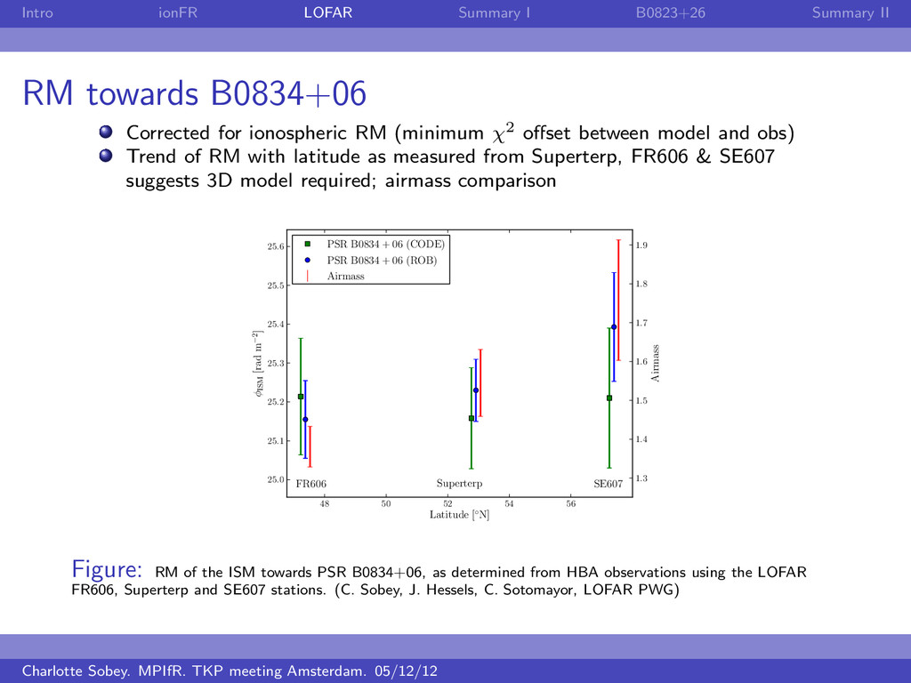
    RM towards B0834+06
    Corrected for ionospheric RM (minimum χ2 offset between model and obs)
    Trend of RM with latitude as measured from Superterp, FR606 & SE607
    suggests 3D model required; airmass comparison
    48 50 52 54 56
    Latitude [◦N]
    25.0
    25.1
    25.2
    25.3
    25.4
    25.5
    25.6
    φISM
    [rad m−2]
    1.3
    1.4
    1.5
    1.6
    1.7
    1.8
    1.9
    Airmass
    Superterp
    FR606 SE607
    PSR B0834 + 06 (CODE)
    PSR B0834 + 06 (ROB)
    Airmass
    Figure: RM of the ISM towards PSR B0834+06, as determined from HBA observations using the LOFAR
    FR606, Superterp and SE607 stations. (C. Sobey, J. Hessels, C. Sotomayor, LOFAR PWG)
    Charlotte Sobey. MPIfR. TKP meeting Amsterdam. 05/12/12
    

    View Slide

13. Intro ionFR LOFAR Summary I B0823+26 Summary II
    Summary I
    Observing pulsars in polarisation interesting, in particular to derive magnetic
    field of Milky Way
    Need to correct for ionospheric contribution, especially if monitoring RMs over
    long timescales (years)
    ionFR can predict ionospheric Faraday rotation
    Comparisons between the model and observations seem very good, higher time
    resolution and finer gridding for TEC maps better
    LOFAR can measure high-precision RMs, calibrate for ionosphere using ionFR –
    in future 3D modelling
    Bring on cycle 0 observations! 2/3 observations of pulsars with known and
    unknown RMs
    Charlotte Sobey. MPIfR. TKP meeting Amsterdam. 05/12/12
    

    View Slide

14. Intro ionFR LOFAR Summary I B0823+26 Summary II
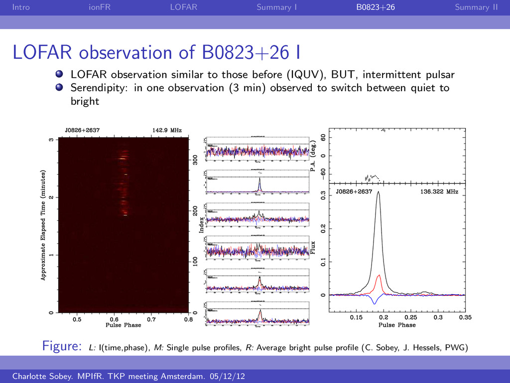
    LOFAR observation of B0823+26 I
    LOFAR observation similar to those before (IQUV), BUT, intermittent pulsar
    Serendipity: in one observation (3 min) observed to switch between quiet to
    bright
    Figure: L: I(time,phase), M: Single pulse profiles, R: Average bright pulse profile (C. Sobey, J. Hessels, PWG)
    Charlotte Sobey. MPIfR. TKP meeting Amsterdam. 05/12/12
    

    View Slide

15. Intro ionFR LOFAR Summary I B0823+26 Summary II
    LOFAR observation of B0823+26 II
    LOFAR observation in total intensity (3 hr, HBA, 48 MHz, I)
    Again, in one observation, switch between quiet to bright mode
    Interesting: previously thought ‘off’ mode actually just ‘quiet’ (emission still
    present)
    Figure: L: I(time,phase) quiet mode, M: I(time,phase) bright mode, R: Single pulse profiles (C. Sobey, J.
    Hessels, LOFAR PWG)
    Charlotte Sobey. MPIfR. TKP meeting Amsterdam. 05/12/12
    

    View Slide

16. Intro ionFR LOFAR Summary I B0823+26 Summary II
    LOFAR observation of B0823+26 II
    LOFAR observation in total intensity (3 hr, HBA, 48 MHz, I)
    Differences between quiet and bright modes: pulse profile distributions
    0.40 0.45 0.50 0.55
    Pulse phase of peak profile
    50
    100
    150
    200
    250
    300
    No. single pulses
    B
    Q
    Figure: L: Average pulse profile quiet (black) & bright (red) modes, R: Histogram of location of peak in single
    pulse profiles quiet (red) & bright (blue) modes, (C. Sobey, J. Hessels, LOFAR PWG)
    Charlotte Sobey. MPIfR. TKP meeting Amsterdam. 05/12/12
    

    View Slide

17. Intro ionFR LOFAR Summary I B0823+26 Summary II
    Summary II
    Two rare observations during mode change of PSR B0823+26 (esp. with
    polarisation)
    High sensitivity of LOFAR allowed detection of pulse in previously thought ‘off’
    mode
    Provides information about magnetosphere emission – how to produce mode
    change within a single pulse?
    Rapid change in magnetic field and/or electron density?
    Thank you for listening!
    Charlotte Sobey. MPIfR. TKP meeting Amsterdam. 05/12/12
    

    View Slide