Redshift-space distortions

Redshift space distortions in statistical descriptions of density field.

Transcript

1. Redshift-space distortions Vikrant Kamble August 15, 2017
2. Doppler shift: ∆λ λ = v c Using cosmological redshift to measure distances gives: ∆λ λ = vH c = aHx c What if velocity has additional contributions → what we will be measuring in position in redshift-space ∆λ λ = vH + vpec c = aHs c Using the above two equations and making plane-parallel approximation with z-axis along LOS, we get s = x + vpec z aH ˆ z = x + upec z ˆ z Where we see is not where it actually is!
3. By mass conversation we must have: (1 + δs g )d3s = (1 + δx g )d3x d3s = d3x 1 + duz (x) dz
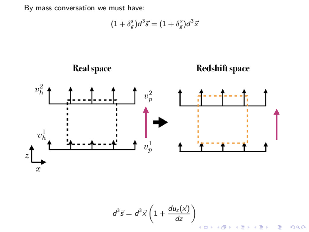
4. From last two equations, we have 1 + δs g = (1 + δx g ) 1 + duz (x) dz −1 (1) In analogy to electrostatics, the divergence of the velocity field at any point is due to some source density at that point. ∇ · u(x) = −θ Just like conservative electric field we assume that the velocity field in real space is irrotational. ∇ × u(x) = 0 → u(x) = ∇λ Taking the divergence of the above equation gives: ∇ · ∇λ = div(gradλ) = laplacian λ = −θ λ = −∇−2θ = −inv.laplacian θ This whole shebang is to allow us to write the duz (x)/dz in eq. 1 in terms of source density θ.
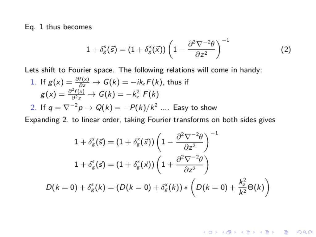
5. Eq. 1 thus becomes 1 + δs g (s) = (1 + δx g (x)) 1 − ∂2∇−2θ ∂z2 −1 (2) Lets shift to Fourier space. The following relations will come in handy: 1. If g(x) = ∂f (x) ∂z → G(k) = −ikz F(k), thus if g(x) = ∂2f (x) ∂2z → G(k) = −k2 z F(k) 2. If q = ∇−2p → Q(k) = −P(k)/k2 .... Easy to show Expanding 2. to linear order, taking Fourier transforms on both sides gives 1 + δs g (s) = (1 + δx g (x)) 1 − ∂2∇−2θ ∂z2 −1 1 + δs g (s) = (1 + δx g (x)) 1 + ∂2∇−2θ ∂z2 D(k = 0) + δs g (k) = (D(k = 0) + δx g (k)) ∗ D(k = 0) + k2 z k2 Θ(k)
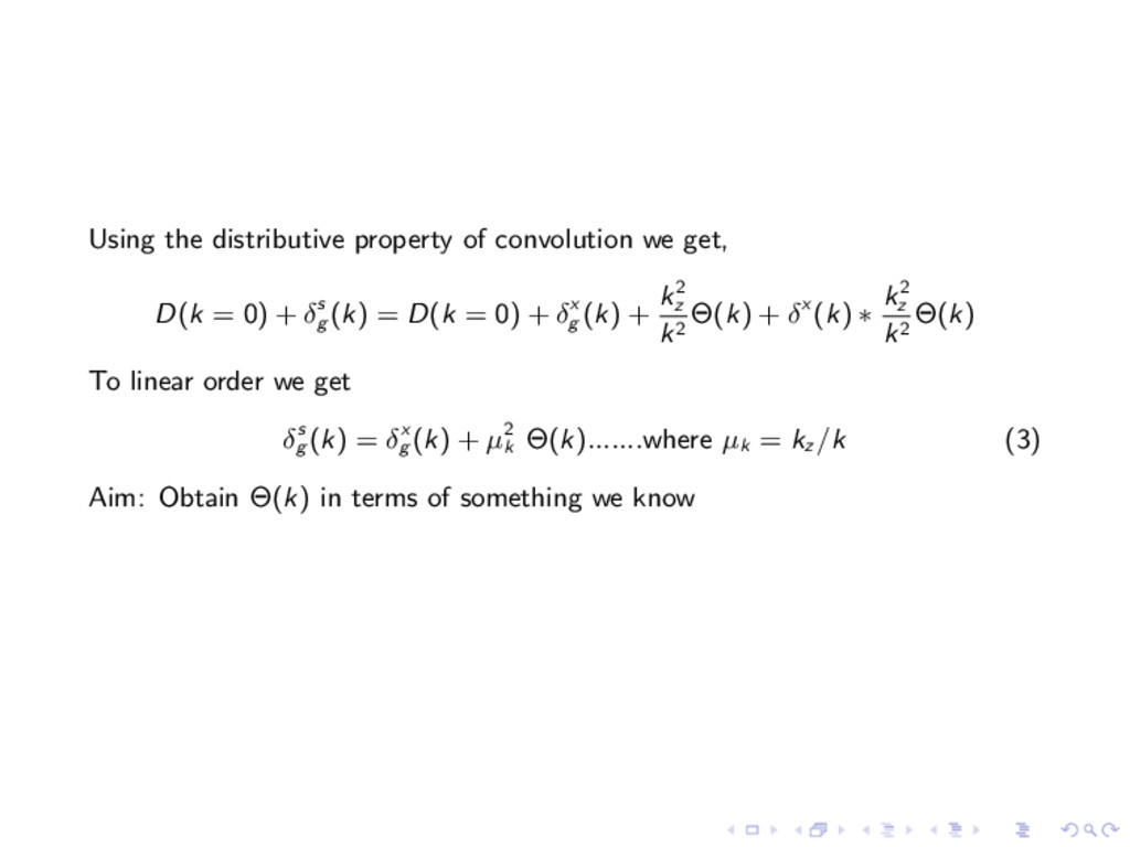
6. Using the distributive property of convolution we get, D(k = 0) + δs g (k) = D(k = 0) + δx g (k) + k2 z k2 Θ(k) + δx (k) ∗ k2 z k2 Θ(k) To linear order we get δs g (k) = δx g (k) + µ2 k Θ(k).......where µk = kz /k (3) Aim: Obtain Θ(k) in terms of something we know
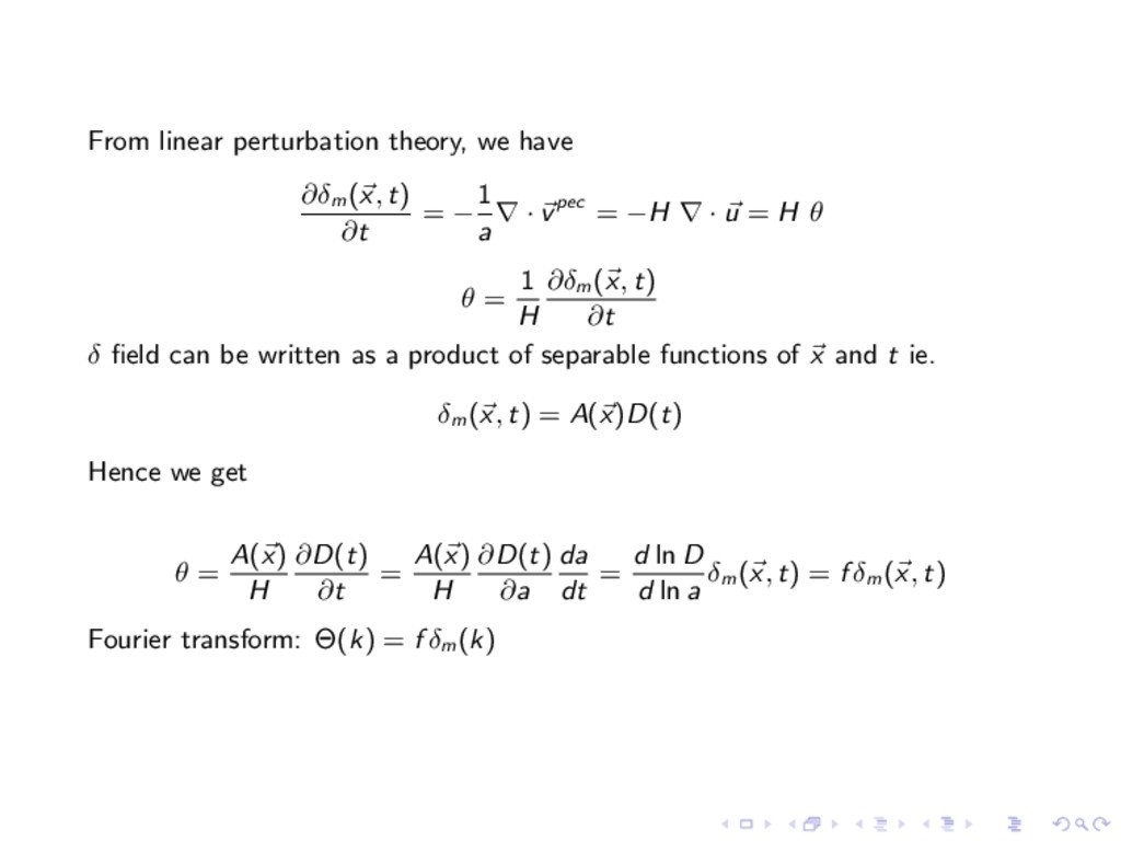
7. From linear perturbation theory, we have ∂δm (x, t) ∂t = − 1 a ∇ · vpec = −H ∇ · u = H θ θ = 1 H ∂δm (x, t) ∂t δ field can be written as a product of separable functions of x and t ie. δm (x, t) = A(x)D(t) Hence we get θ = A(x) H ∂D(t) ∂t = A(x) H ∂D(t) ∂a da dt = d ln D d ln a δm (x, t) = f δm (x, t) Fourier transform: Θ(k) = f δm (k)
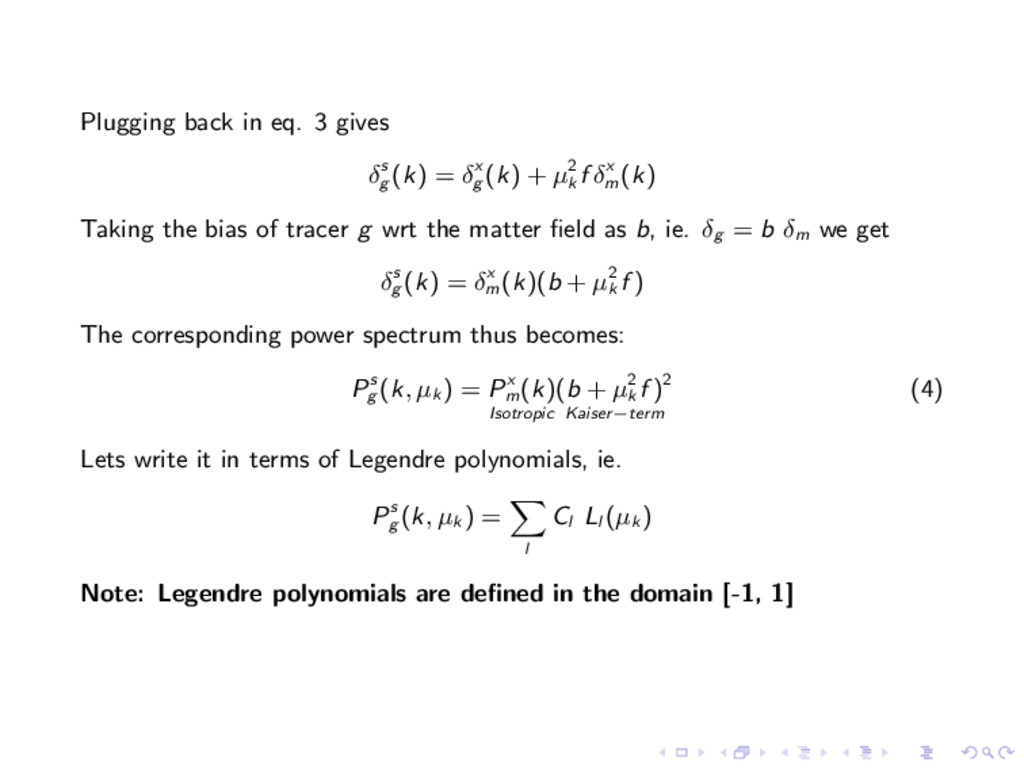
8. Plugging back in eq. 3 gives δs g (k) = δx g (k) + µ2 k f δx m (k) Taking the bias of tracer g wrt the matter field as b, ie. δg = b δm we get δs g (k) = δx m (k)(b + µ2 k f ) The corresponding power spectrum thus becomes: Ps g (k, µk ) = Px m (k) Isotropic (b + µ2 k f )2 Kaiser−term (4) Lets write it in terms of Legendre polynomials, ie. Ps g (k, µk ) = l Cl Ll (µk ) Note: Legendre polynomials are defined in the domain [-1, 1]
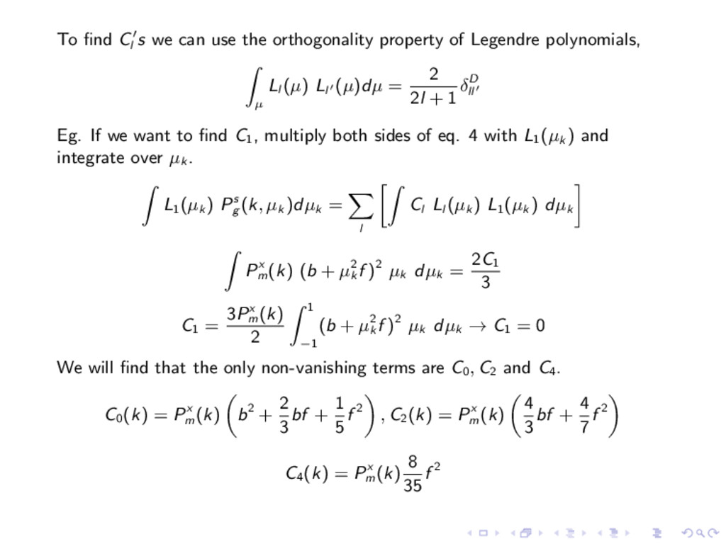
9. To find Cl s we can use the orthogonality property of Legendre polynomials, µ Ll (µ) Ll (µ)dµ = 2 2l + 1 δD ll Eg. If we want to find C1 , multiply both sides of eq. 4 with L1 (µk ) and integrate over µk . L1 (µk ) Ps g (k, µk )dµk = l Cl Ll (µk ) L1 (µk ) dµk Px m (k) (b + µ2 k f )2 µk dµk = 2C1 3 C1 = 3Px m (k) 2 1 −1 (b + µ2 k f )2 µk dµk → C1 = 0 We will find that the only non-vanishing terms are C0, C2 and C4 . C0 (k) = Px m (k) b2 + 2 3 bf + 1 5 f 2 , C2 (k) = Px m (k) 4 3 bf + 4 7 f 2 C4 (k) = Px m (k) 8 35 f 2
10. Correlation function is the Inverse Fourier Transform of the Power Spectrum. ξs g (r) = 1 (2π)3 Vk d3k eik·r Ps (k) = 1 (2π)3 Vk k2 dk dµk dφk eik·r l Cl (k) Ll (µk ) = 1 (2π)3 l Vk k2 dk dµk dφk eik·r Cl (k) Ll (µk ) = 1 (2π)3 l   k k2 dk Cl (k) dΩk eikr cos γLl (µk ) How to evaluate?  
11. Rayleigh expansion of spherical waves: eik·r = l il (2l + 1) jl (kr) Ll (cos γ) Plugging this in above equation gives: ξs g (r) = 1 (2π)3 l k k2 dk Cl (k) dΩk l il (2l + 1) jl (kr) Ll (cos γ) Ll (µk ) = 1 (2π)3 l l il (2l + 1) k k2 dk Cl (k) jl (kr) dΩk Ll (cos γ) Ll (µk ) It can be shown that dΩk Ll (cos γ) Ll (µk ) = 4π 2l + 1 Ll (µr ) δD ll This gives ξs g (r) = ξs g (r, µr ) = l k k2 dk jl (kr) Cl (k) 2π2 Ll (µr )