Gaussian Process

Transcript

1. Gaussian Random Fields Vikrant Kamble September 28, 2017 Vikrant Kamble Gaussian Random Fields September 28, 2017 1 / 13
2. Univariate Gaussian f (x) = 1 √ 2πσ2 exp − (x − µ)2 2σ2 ndim = 1, µ = µx , C = [σ2 x ] Vikrant Kamble Gaussian Random Fields September 28, 2017 2 / 13
3. Bivariate Gaussian f (x, y) = 1 2πσx σy 1 − ρ2 exp − 1 2(1 − ρ2) (x − µx )2 σ2 x + (y − µy )2 σ2 y − 2ρ(x − µx )(y − µy ) σx σy (1) ndim = 2, µ = [µx , µy ], C = σ2 x σxy σxy σ2 y , ρ = σxy σx σy Vikrant Kamble Gaussian Random Fields September 28, 2017 3 / 13
4. Multivariate Gaussian f (x1, x2, ...xn ) = 1 (2π)k |C| exp − 1 2 (x − µ)C−1(x − µ)T ndim = n, µ = [µ1, µ2, ...µn ], C =     σ2 1 σ12 σ13 ... σ21 σ2 2 σ23 ... σ31 σ32 σ2 3 ... ... ... ... σ2 n     To simulate this, we need n (mean) + n 2 covariance parameters Vikrant Kamble Gaussian Random Fields September 28, 2017 4 / 13
5. Scalar field Def: A scalar field is a function over space that maps each location to a real value. f : Rn → R e.g. Higgs field, δ field Vikrant Kamble Gaussian Random Fields September 28, 2017 5 / 13
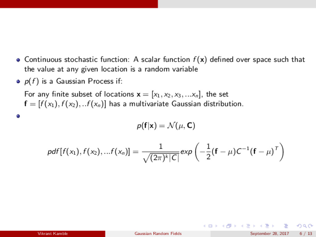
6. Continuous stochastic function: A scalar function f (x) defined over space such that the value at any given location is a random variable p(f ) is a Gaussian Process if: For any finite subset of locations x = [x1, x2, x3, ...xn ], the set f = [f (x1 ), f (x2 ), ..f (xn )] has a multivariate Gaussian distribution. p(f|x) = N(µ, C) pdf [f (x1 ), f (x2 ), ...f (xn )] = 1 (2π)k |C| exp − 1 2 (f − µ)C−1(f − µ)T Vikrant Kamble Gaussian Random Fields September 28, 2017 6 / 13
7. To simulate a GP, all we need is a mean function µ(x) and a Kernel K(xi , xj ) that allows us to construct the Covariance matrix C. p(f |X) = N(0, K) A Kernel is a function that takes a pair of vectors and maps them to a scalar quantity K(xi , xj ) : Rn × Rn → R Let’s simulate!!! Vikrant Kamble Gaussian Random Fields September 28, 2017 7 / 13
8. 1D: White Kernel µ(x) = 0, K(xi , xj ) = σ2δij 0 10 f(x) 0 10 f(x) 2 4 6 8 10 x 0 10 f(x) No structure ξ(r) = 0 ∀ r > 0 Vikrant Kamble Gaussian Random Fields September 28, 2017 8 / 13
9. 1D: ExpSquared Kernel Also known as the Radial Basis function (RBF) Kernel µ(x) = 0, K(xi , xj ; rc ) = exp −(xi − xj )2 2r2 c = exp −r2 2r2 c −2 0 2 f(x) rc = 0.5 −2 0 2 f(x) rc = 1.0 0.0 2.5 5.0 7.5 10.0 x −2 0 2 f(x) rc = 2.0 rc also known as bandwidth defines the char- acteristic scale of clustering. Vikrant Kamble Gaussian Random Fields September 28, 2017 9 / 13
10. 1D: Other Kernels Matern32-Kernel: K = 1 + 3r ρ exp − √ 3r ρ −2 0 2 f(x) ρ = 2.0 −2 0 2 f(x) ρ = 6.0 0.0 2.5 5.0 7.5 10.0 x −2 0 2 f(x) ρ = 8.0 Exponential-Kernel: K = exp − r ρ −2 0 2 f(x) ρ = 1.0 −2 0 2 f(x) ρ = 4.0 0.0 2.5 5.0 7.5 10.0 x −2 0 2 f(x) ρ = 8.0 Cosine-Kernel: K = cos 2π r T −2 0 2 f(x) T = 1.0 −2 0 2 f(x) T = 4.0 0.0 2.5 5.0 7.5 10.0 x −2 0 2 f(x) T = 8.0 Vikrant Kamble Gaussian Random Fields September 28, 2017 10 / 13
11. For the perturbation field, we have pdf [δ(x1 ), δ(x2 ), ...δ(xn )] = 1 (2π)k |C| exp − 1 2 δ C−1δT The kernel K is nothing but the correlation function ξ(r). Assuming that the Universe is homogeneous, isotropic and all n > 2-point correlation functions vanish, the only quantity we need to fully capture all the information of the Universe is ξ(r). Redshift Space Distortions (RSD) - ξ(r) → ξ(r, θ). Non-gaussianity → finite (n > 2)-point correlation functions Vikrant Kamble Gaussian Random Fields September 28, 2017 11 / 13
12. Our Universe is just one realization of a Gaussian Process. Figure: Planck CMB Map 1 1http://sci.esa.int/science-e-media/img/61/PlanckC MBM ollweide4k.jpg Vikrant Kamble Gaussian Random Fields September 28, 2017 12 / 13
13. The Machinery: First pick the locations x1, x2, ..., xn Remember, the probability distribution is over the scalar field value at these chosen locations, and not the location themselves. Create the mean vector of the perturbations µ = [g(x1 ), g(x2 ), ..., g(xn )] At early Universe, µ = 0 Create the Covariance matrix using the kernel. For the perturbation field K(xi , xj ; θ) = K(|xi − xj |; θ) = ξ(r; θ) What we have is f ∼ N(g(x)N , CN×N ) Sample once to get one realization of the function Vikrant Kamble Gaussian Random Fields September 28, 2017 13 / 13