EM algorithm

Transcript

1. EM Algorithm 2014/11/14 Yuichiro Tsuchiya
2. Introduction with GMM
3. Example: Gaussian Mixture Models Given data points…
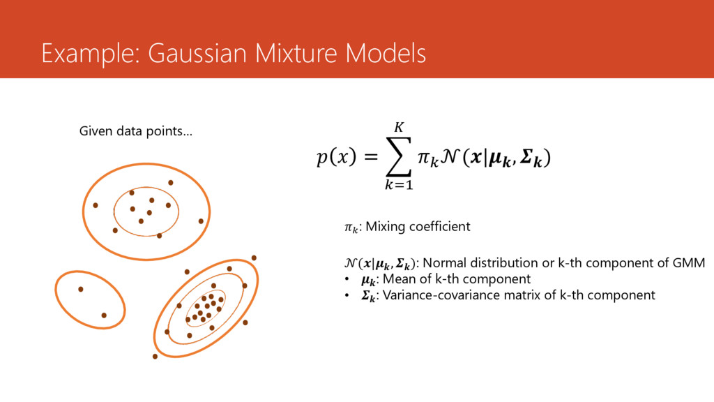
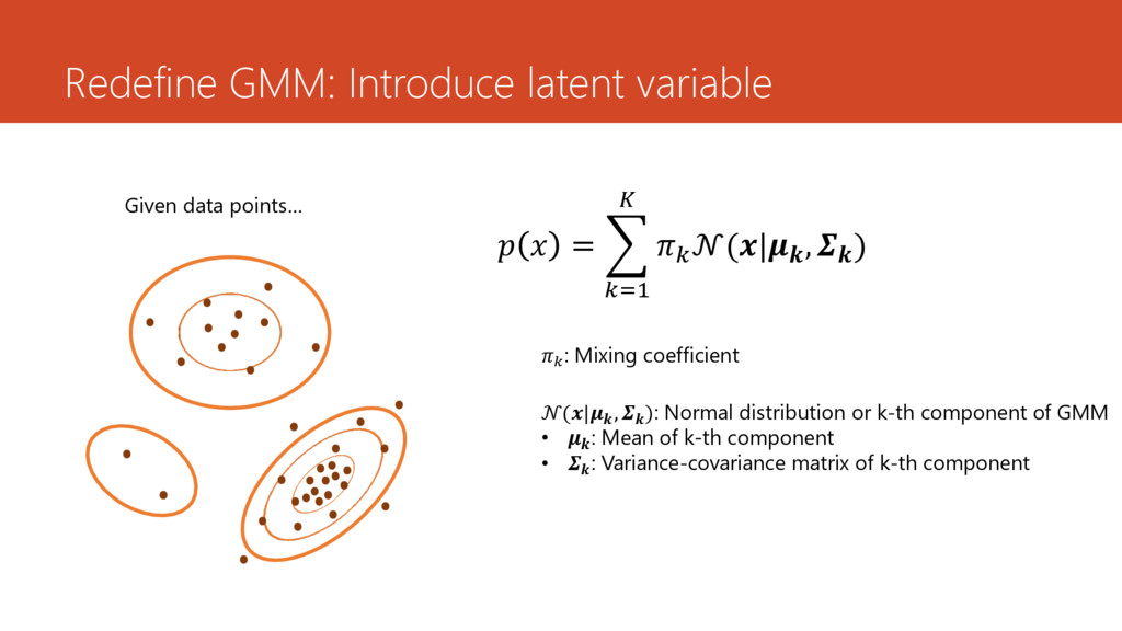
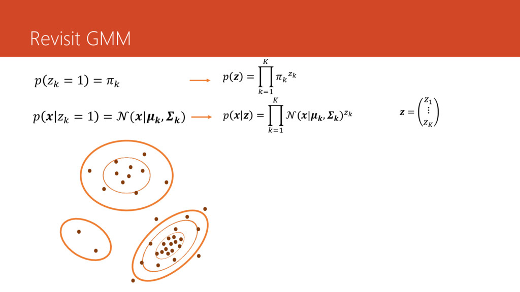
4. Example: Gaussian Mixture Models Given data points… = =1 (| , ) : Mixing coefficient (| , ): Normal distribution or k-th component of GMM • : Mean of k-th component • : Variance-covariance matrix of k-th component
5. How to fit GMM to given data points? = =1 (| , ) Parameters to be determined: , , Maximum likelihood estimation Maximize a log likelihood function ln () ln , , = =1 ln =1 ( | , ) In this case: ( is a set of given data) Likelihood function: Bayes’ theorem: ∝ | ∝ ℎ × | = =1 ( |) in this case: | , = =1 ( | , ) = =1 =1 ( | , )
6. Solve maximum likelihood estimation ln , , = =1 ln =1 (| , )
7. Solve maximum likelihood estimation ln , , = =1 ln =1 (| , ) ln , , = 0 ln , , = 0 ln , , = 0 = 1 =1 ( ) = 1 =1 − − = = =1 ( ) where = (| , ) =1 (| , ) Responsibility that component takes for ‘explaining’ the observation
8. Optimization = 1 =1 ( ) = 1 =1 − − = = =1 ( ) where = (| , ) =1 (| , ) , , and depend on each other No closed-form solution
9. Optimization = 1 =1 ( ) = 1 =1 − − = = =1 ( ) where = (| , ) =1 (| , ) , , and depend on each other No closed-form solution
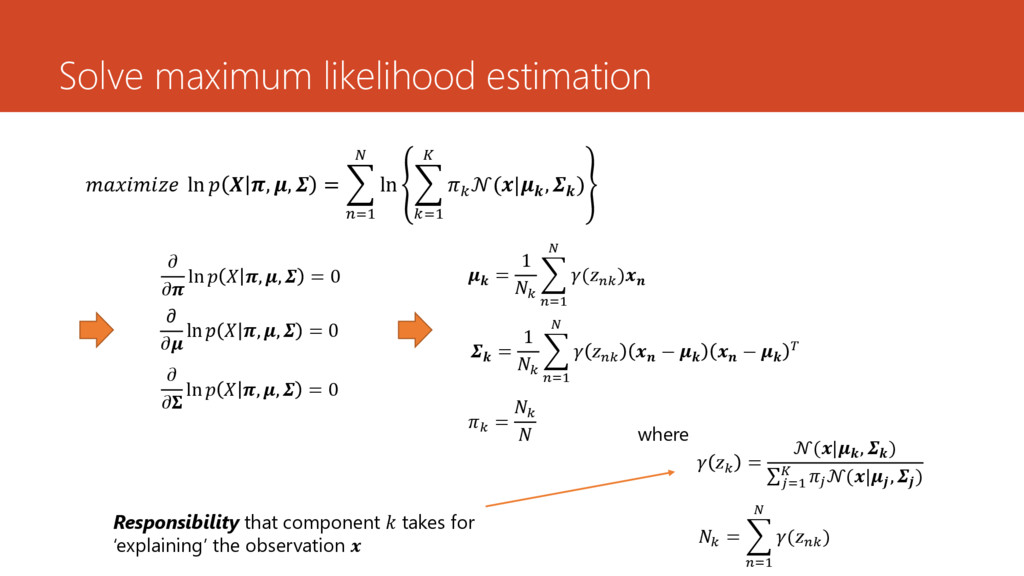
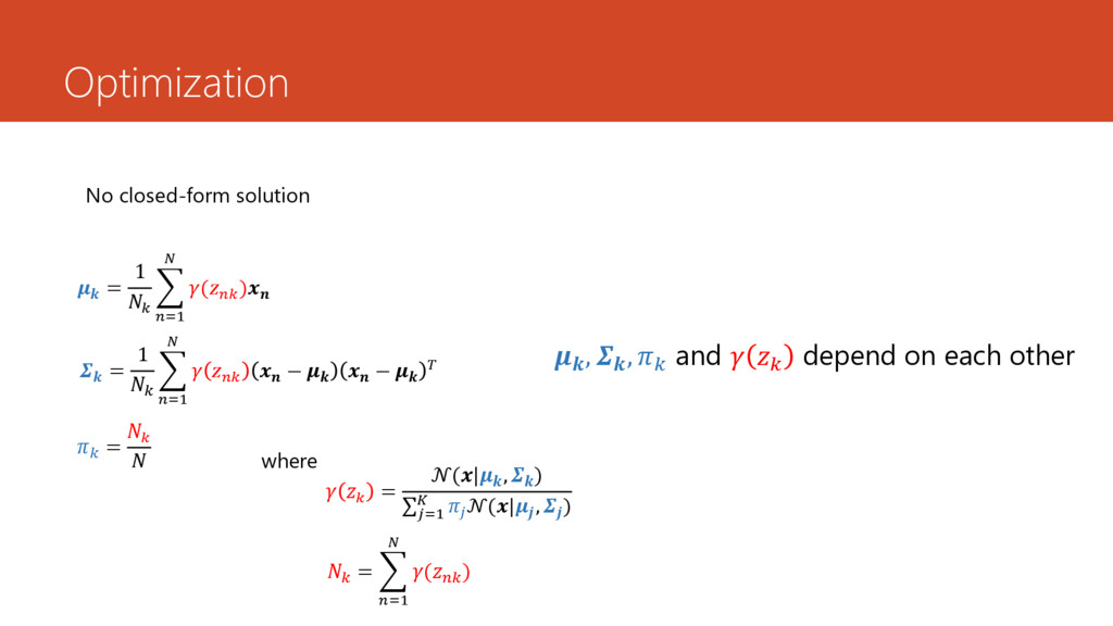
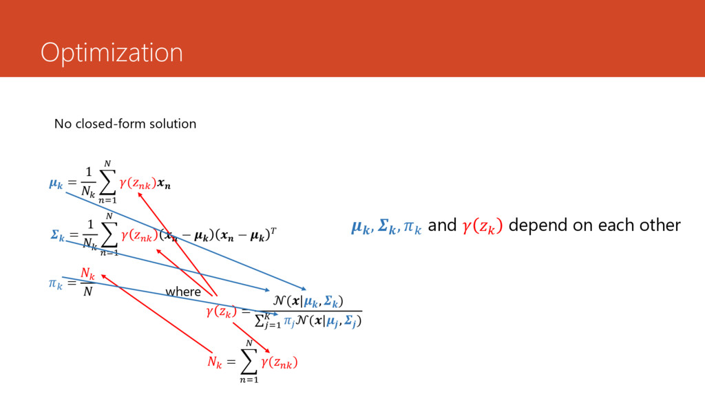
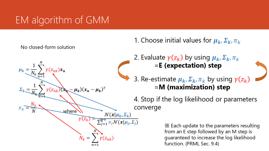
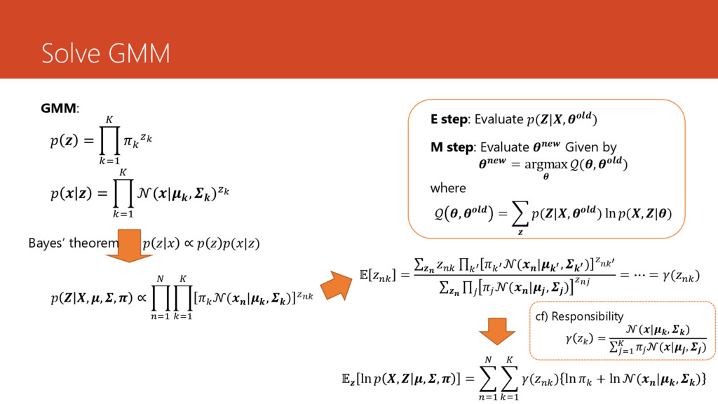
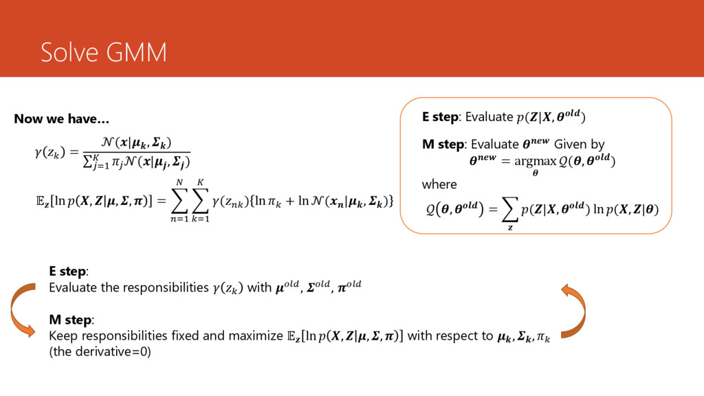
10. EM algorithm of GMM 1. Choose initial values for , , 2. Evaluate by using , , =E (expectation) step 3. Re-estimate , , by using =M (maximization) step = 1 =1 ( ) = 1 =1 − − = = =1 ( ) where = (| , ) =1 (| , ) No closed-form solution ※ Each update to the parameters resulting from an E step followed by an M step is guaranteed to increase the log likelihood function. (PRML Sec. 9.4) 4. Stop if the log likelihood or parameters converge
11. Introduce latent variables
12. Redefine GMM: Introduce latent variable Given data points… = =1 (| , ) : Mixing coefficient (| , ): Normal distribution or k-th component of GMM • : Mean of k-th component • : Variance-covariance matrix of k-th component
13. Redefine GMM: Introduce latent variable = =1 (| , ) Introduce latent variable = 1 = ( = 1 (Probability)) = =1 = 1 = (| , ) latent variable is… • = 1 , 2 , ⋯ , • ∈ 0,1 • = 1 (1-of-K representation) (Assign just 1 component) another representation = =1 (| , )
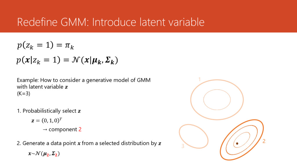
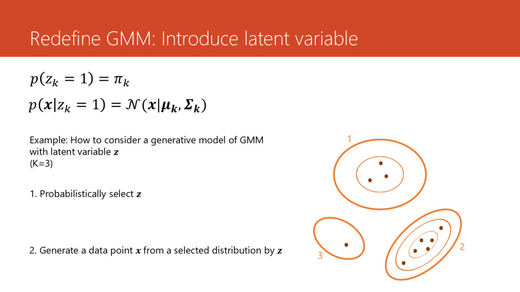
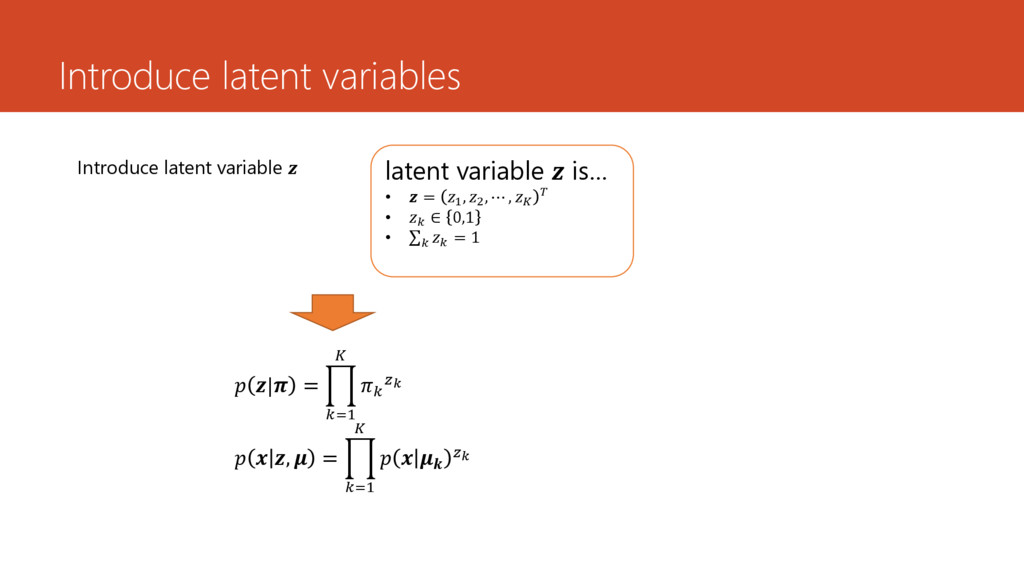
14. 3 2 Redefine GMM: Introduce latent variable = 1 = = 1 = (| , ) Example: How to consider a generative model of GMM with latent variable (K=3) 1. Probabilistically select = 0, 1, 0 2. Generate a data point from a selected distribution by ~( , ) → component 2 1
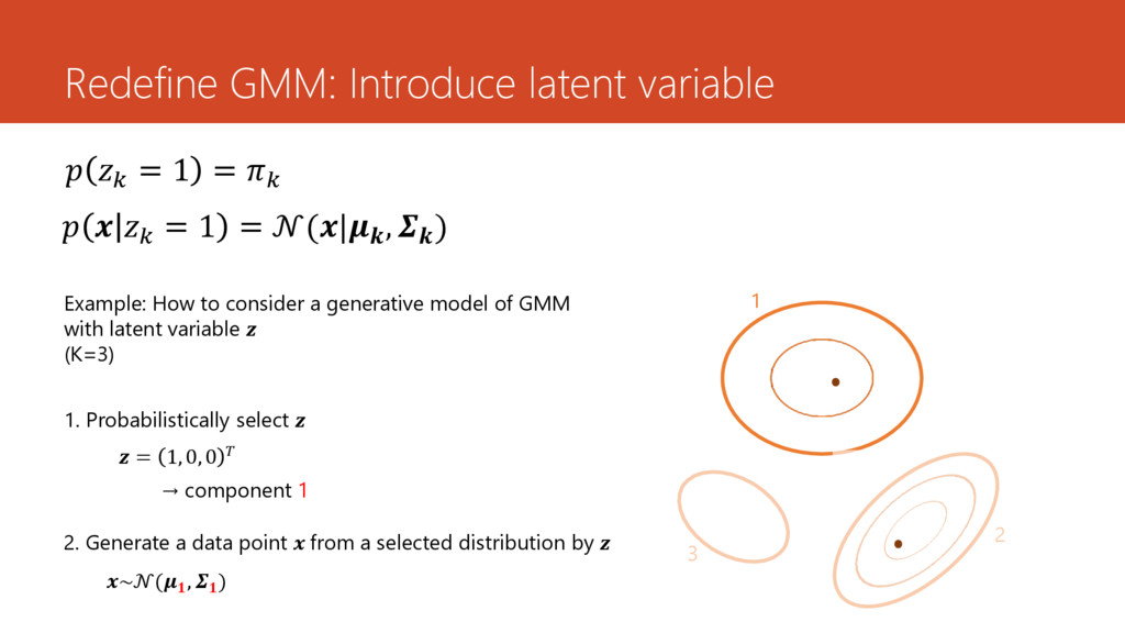
15. 3 2 Redefine GMM: Introduce latent variable = 1 = = 1 = (| , ) Example: How to consider a generative model of GMM with latent variable (K=3) 1. Probabilistically select = 1, 0, 0 2. Generate a data point from a selected distribution by ~( , ) → component 1 1
16. 3 2 Redefine GMM: Introduce latent variable = 1 = = 1 = (| , ) Example: How to consider a generative model of GMM with latent variable (K=3) 1. Probabilistically select 2. Generate a data point from a selected distribution by 1
17. EM algorithm for latent variable models
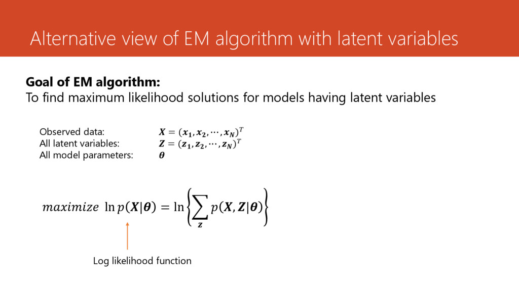
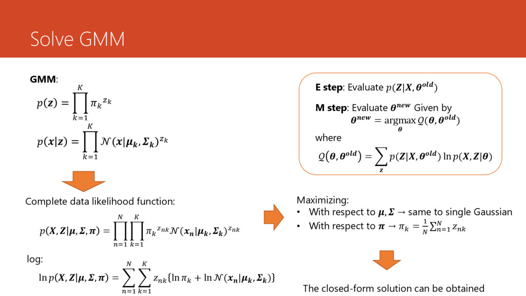
18. Alternative view of EM algorithm with latent variables Goal of EM algorithm: To find maximum likelihood solutions for models having latent variables Observed data: = ( , , ⋯ , ) All latent variables: = ( , , ⋯ , ) All model parameters: ln | = ln , | Log likelihood function
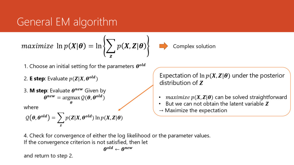
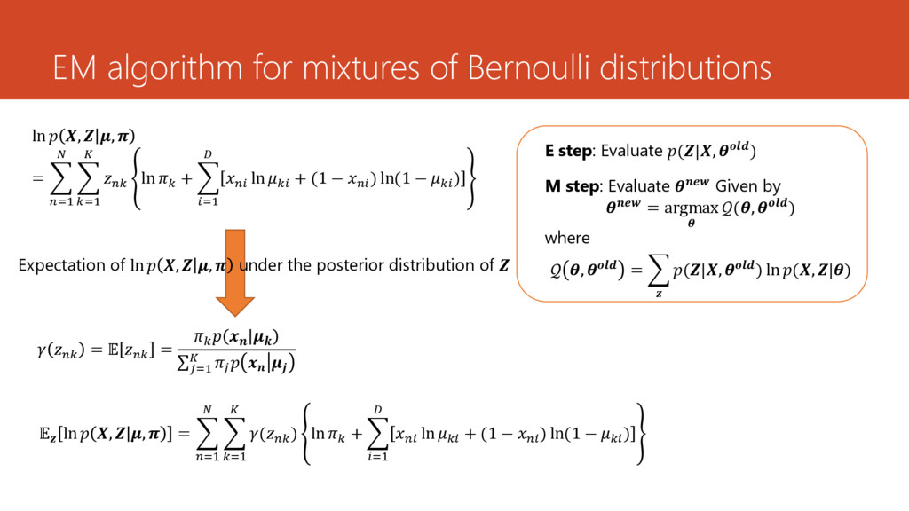
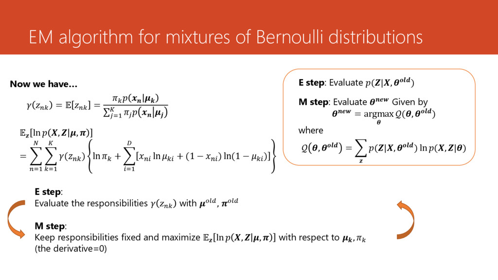
19. General EM algorithm 1. Choose an initial setting for the parameters 2. E step: Evaluate (|, ) 3. M step: Evaluate Given by = argmax (, ) where , = (|, ) ln (, |) 4. Check for convergence of either the log likelihood or the parameter values. If the convergence criterion is not satisfied, then let ← and return to step 2. ln | = ln , | Expectation of ln (, |) under the posterior distribution of Complex solution • (, |) can be solved straightforward • But we can not obtain the latent variable → Maximize the expectation
20. Revisit GMM = 1 = = 1 = (| , ) = =1 = =1 (| , ) = 1 ⋮
21. Solve GMM E step: Evaluate (|, ) M step: Evaluate Given by = argmax (, ) where , = (|, ) ln (, |) = =1 = =1 (| , ) GMM: Complete data likelihood function: , , , = =1 =1 ( | , ) Maximizing: • With respect to , → same to single Gaussian • With respect to → = 1 =1 The closed-form solution can be obtained ln , , , = =1 =1 ln + ln ( | , ) log:
22. Solve GMM ∝ (|) Bayes’ theorem , , , ∝ =1 =1 ( | , ) = =1 = =1 (| , ) GMM: E step: Evaluate (|, ) M step: Evaluate Given by = argmax (, ) where , = (|, ) ln (, |) = ′ ′( |′, ′) ′ ( | , ) = ⋯ = ( ) ln , , , = =1 =1 ( ) ln + ln ( | , ) = (| , ) =1 (| , ) cf) Responsibility
23. Solve GMM Now we have… ln , , , = =1 =1 ( ) ln + ln ( | , ) = (| , ) =1 (| , ) E step: Evaluate (|, ) M step: Evaluate Given by = argmax (, ) where , = (|, ) ln (, |) E step: Evaluate the responsibilities with , , M step: Keep responsibilities fixed and maximize ln , , , with respect to , , (the derivative=0)
24. Analogy: k-means GMM k-means
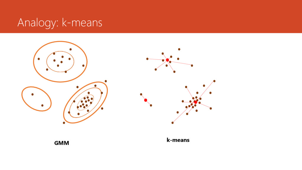
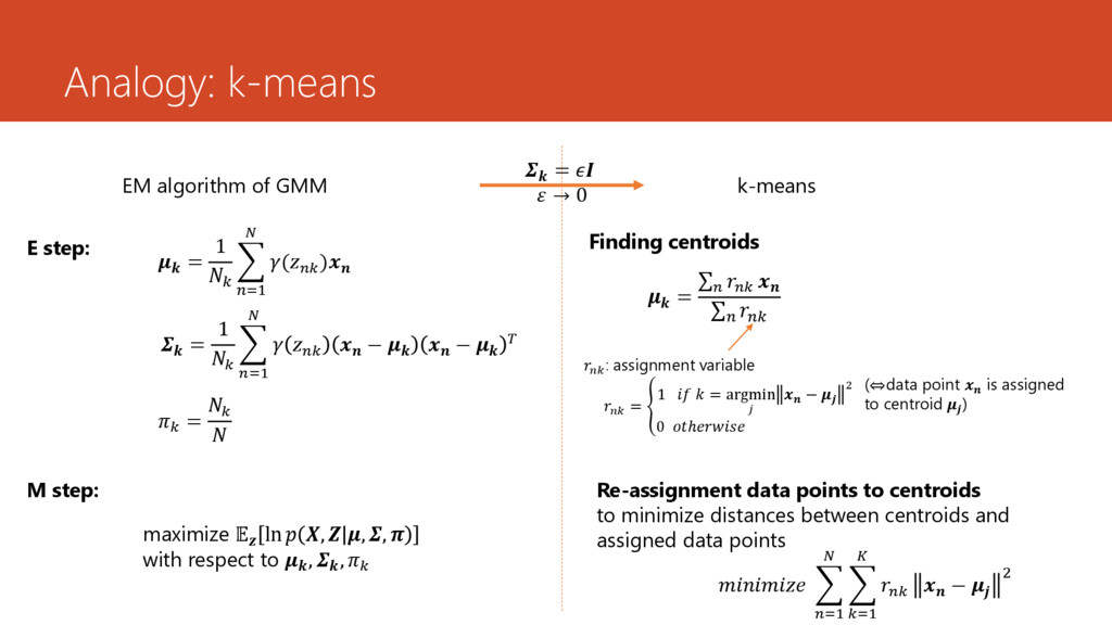
25. Analogy: k-means EM algorithm of GMM k-means = 1 =1 ( ) = 1 =1 − − = E step: Finding centroids M step: maximize ln , , , with respect to , , Re-assignment data points to centroids to minimize distances between centroids and assigned data points = → 0 = : assignment variable = 1 = argmin − 2 0 ℎ =1 =1 − 2 (⇔data point is assigned to centroid )
26. Mixtures of Bernoulli distributions
27. Another applications of EM algorithm Mixtures of Bernoulli distributions binary variables ( = 1, … , ) = =1 (1 − )(1−) (Bernoulli distribution with parameter ) = 1 , 2 , … , = 1 , 2 , … , Let’s consider a finite mixture of these distributions: , = =1 , = =1 (1 − )(1−) = 1 , 2 , … , = 1 , 2 , … ,
28. Mixtures of Bernoulli distributions , = =1 , = =1 (1 − )(1−) = 1 , 2 , … , = 1 , 2 , … , Let’s determine parameters when data points = , , … , given Maximize the log likelihood function ln , = =1 ln =1 No closed-form solution… →EM algorithm!
29. Introduce latent variables Introduce latent variable latent variable is… • = 1 , 2 , ⋯ , • ∈ 0,1 • = 1 , = =1 | = =1
30. EM algorithm for mixtures of Bernoulli distributions E step: Evaluate (|, ) M step: Evaluate Given by = argmax (, ) where , = (|, ) ln (, |) ln , , = =1 =1 ( ) ln + =1 ln + (1 − ) ln(1 − ) = = =1 ln , , = =1 =1 ln + =1 ln + (1 − ) ln(1 − ) Expectation of ln , , under the posterior distribution of
31. EM algorithm for mixtures of Bernoulli distributions Now we have… E step: Evaluate the responsibilities with , M step: Keep responsibilities fixed and maximize ln , , with respect to , (the derivative=0) E step: Evaluate (|, ) M step: Evaluate Given by = argmax (, ) where , = (|, ) ln (, |) ln , , = =1 =1 ( ) ln + =1 ln + (1 − ) ln(1 − ) = = =1
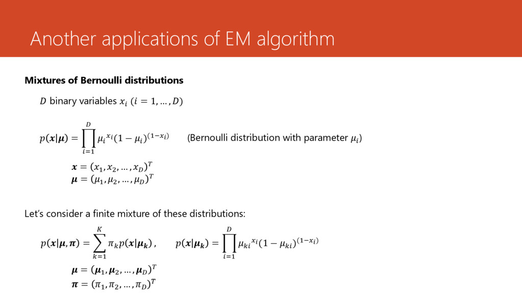
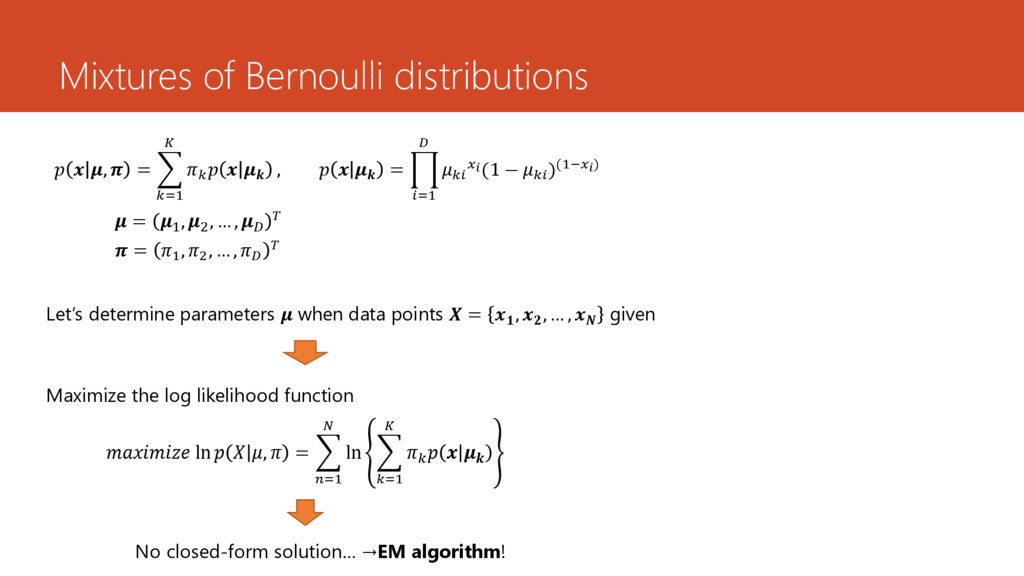
32. Conclusion Goal of EM algorithm is: To find maximum likelihood solutions for models having latent variables For example: • Gaussian Mixture Models • Mixtures of Bernoulli distributions If you want to learn more, see PRML Sec. 9