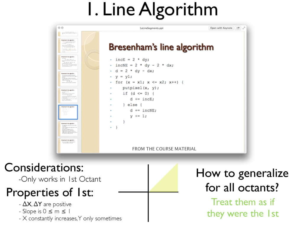
of 1st: - ∆X, ∆Y are positive - Slope is 0 ≤ m ≤ 1 - X constantly increases, Y only sometimes How to generalize for all octants? Treat them as if they were the 1st FROM THE COURSE MATERIAL
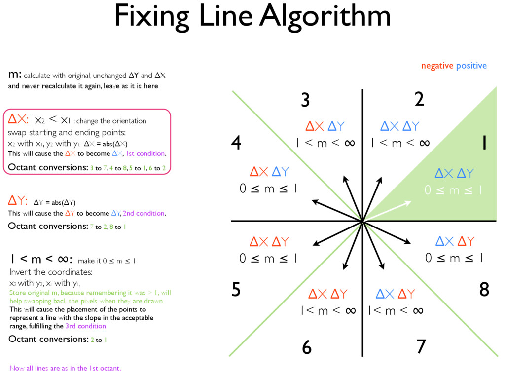
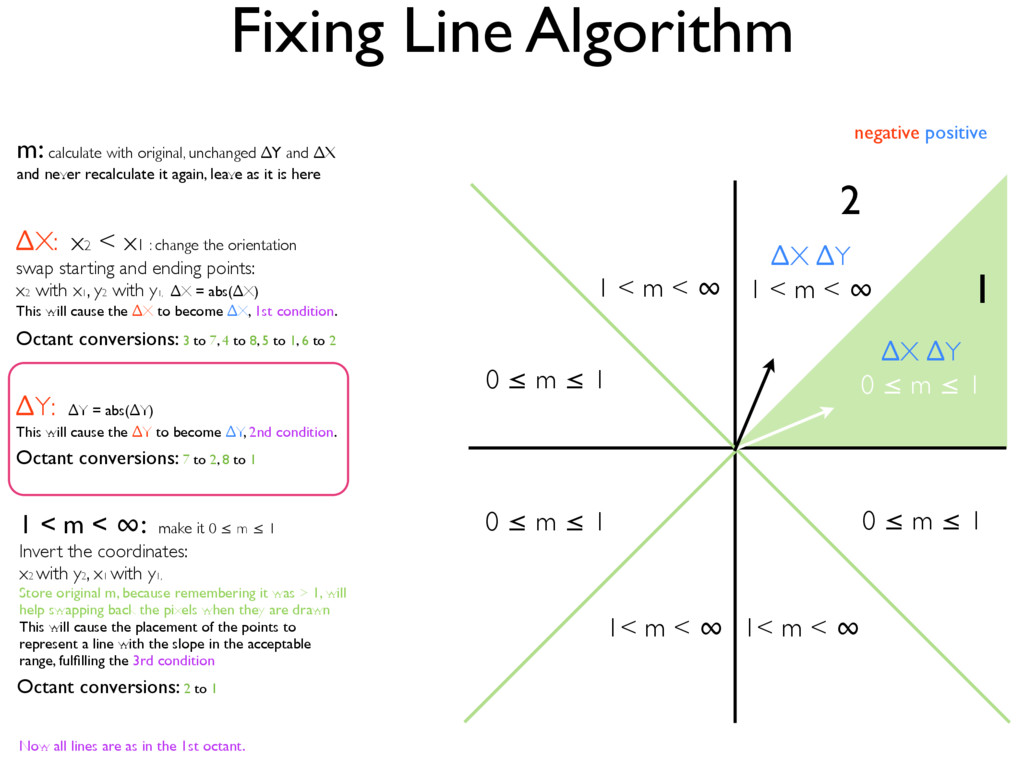
2 3 7 6 4 5 8 1 ∆X ∆Y 1 < m < ∞ ∆X ∆Y 1 < m < ∞ ∆X ∆Y 0 ≤ m ≤ 1 ∆X ∆Y 0 ≤ m ≤ 1 ∆X ∆Y 1< m < ∞ ∆X ∆Y 1< m < ∞ ∆X ∆Y 0 ≤ m ≤ 1 negative positive ∆X: x2 < x1 : change the orientation swap starting and ending points: x2 with x1 , y2 with y1, ∆X = abs(∆X) This will cause the ∆X to become ∆X, 1st condition. 1 < m < ∞: make it 0 ≤ m ≤ 1 Invert the coordinates: x2 with y2 , x1 with y1, Store original m, because remembering it was > 1, will help swapping back the pixels when they are drawn This will cause the placement of the points to represent a line with the slope in the acceptable range, fulfilling the 3rd condition Octant conversions: 3 to 7, 4 to 8, 5 to 1, 6 to 2 Octant conversions: 2 to 1 m: calculate with original, unchanged ∆Y and ∆X and never recalculate it again, leave as it is here ∆Y: ∆Y = abs(∆Y) This will cause the ∆Y to become ∆Y, 2nd condition. Octant conversions: 7 to 2, 8 to 1 Now all lines are as in the 1st octant.
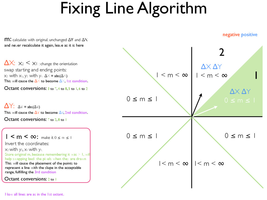
2 3 7 6 4 5 8 1 ∆X ∆Y 1 < m < ∞ ∆X ∆Y 1 < m < ∞ ∆X ∆Y 0 ≤ m ≤ 1 ∆X ∆Y 0 ≤ m ≤ 1 ∆X ∆Y 1< m < ∞ ∆X ∆Y 1< m < ∞ ∆X ∆Y 0 ≤ m ≤ 1 negative positive ∆X: x2 < x1 : change the orientation swap starting and ending points: x2 with x1 , y2 with y1, ∆X = abs(∆X) This will cause the ∆X to become ∆X, 1st condition. 1 < m < ∞: make it 0 ≤ m ≤ 1 Invert the coordinates: x2 with y2 , x1 with y1, Store original m, because remembering it was > 1, will help swapping back the pixels when they are drawn This will cause the placement of the points to represent a line with the slope in the acceptable range, fulfilling the 3rd condition Octant conversions: 3 to 7, 4 to 8, 5 to 1, 6 to 2 Octant conversions: 2 to 1 m: calculate with original, unchanged ∆Y and ∆X and never recalculate it again, leave as it is here ∆Y: ∆Y = abs(∆Y) This will cause the ∆Y to become ∆Y, 2nd condition. Octant conversions: 7 to 2, 8 to 1 Now all lines are as in the 1st octant.
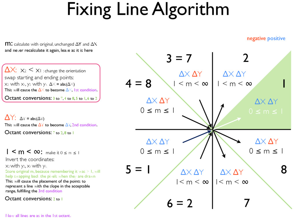
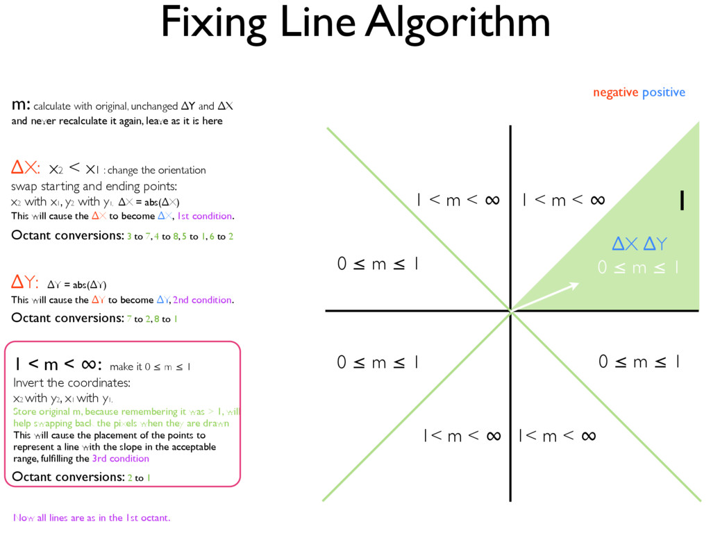
2 3 = 7 7 6 = 2 4 = 8 5 = 1 8 1 ∆X ∆Y 1 < m < ∞ ∆X ∆Y 1 < m < ∞ ∆X ∆Y 0 ≤ m ≤ 1 ∆X ∆Y 0 ≤ m ≤ 1 ∆X ∆Y 1< m < ∞ ∆X ∆Y 1< m < ∞ ∆X ∆Y 0 ≤ m ≤ 1 negative positive ∆X: x2 < x1 : change the orientation swap starting and ending points: x2 with x1 , y2 with y1, ∆X = abs(∆X) This will cause the ∆X to become ∆X, 1st condition. 1 < m < ∞: make it 0 ≤ m ≤ 1 Invert the coordinates: x2 with y2 , x1 with y1, Store original m, because remembering it was > 1, will help swapping back the pixels when they are drawn This will cause the placement of the points to represent a line with the slope in the acceptable range, fulfilling the 3rd condition Octant conversions: 3 to 7, 4 to 8, 5 to 1, 6 to 2 Octant conversions: 2 to 1 m: calculate with original, unchanged ∆Y and ∆X and never recalculate it again, leave as it is here ∆Y: ∆Y = abs(∆Y) This will cause the ∆Y to become ∆Y, 2nd condition. Octant conversions: 7 to 2, 8 to 1 Now all lines are as in the 1st octant.
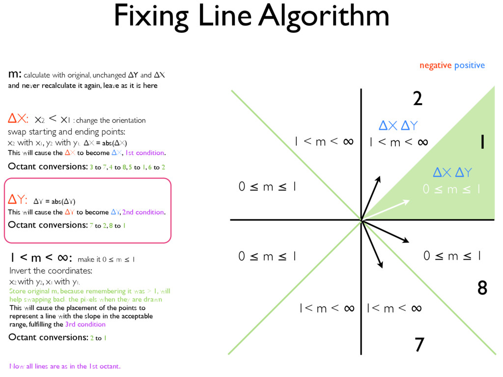
2 7 8 1 ∆X ∆Y 1 < m < ∞ 1< m < ∞ 0 ≤ m ≤ 1 negative positive ∆X: x2 < x1 : change the orientation swap starting and ending points: x2 with x1 , y2 with y1, ∆X = abs(∆X) This will cause the ∆X to become ∆X, 1st condition. 1 < m < ∞: make it 0 ≤ m ≤ 1 Invert the coordinates: x2 with y2 , x1 with y1, Store original m, because remembering it was > 1, will help swapping back the pixels when they are drawn This will cause the placement of the points to represent a line with the slope in the acceptable range, fulfilling the 3rd condition Octant conversions: 3 to 7, 4 to 8, 5 to 1, 6 to 2 Octant conversions: 2 to 1 m: calculate with original, unchanged ∆Y and ∆X and never recalculate it again, leave as it is here ∆Y: ∆Y = abs(∆Y) This will cause the ∆Y to become ∆Y, 2nd condition. Octant conversions: 7 to 2, 8 to 1 Now all lines are as in the 1st octant. ∆X ∆Y 1 < m < ∞ 1 < m < ∞ 0 ≤ m ≤ 1 0 ≤ m ≤ 1 1< m < ∞
2 1 ∆X ∆Y 1 < m < ∞ negative positive ∆X: x2 < x1 : change the orientation swap starting and ending points: x2 with x1 , y2 with y1, ∆X = abs(∆X) This will cause the ∆X to become ∆X, 1st condition. 1 < m < ∞: make it 0 ≤ m ≤ 1 Invert the coordinates: x2 with y2 , x1 with y1, Store original m, because remembering it was > 1, will help swapping back the pixels when they are drawn This will cause the placement of the points to represent a line with the slope in the acceptable range, fulfilling the 3rd condition Octant conversions: 3 to 7, 4 to 8, 5 to 1, 6 to 2 Octant conversions: 2 to 1 m: calculate with original, unchanged ∆Y and ∆X and never recalculate it again, leave as it is here ∆Y: ∆Y = abs(∆Y) This will cause the ∆Y to become ∆Y, 2nd condition. Octant conversions: 7 to 2, 8 to 1 Now all lines are as in the 1st octant. 1< m < ∞ 0 ≤ m ≤ 1 1 < m < ∞ 0 ≤ m ≤ 1 0 ≤ m ≤ 1 1< m < ∞
2 1 ∆X ∆Y 1 < m < ∞ negative positive ∆X: x2 < x1 : change the orientation swap starting and ending points: x2 with x1 , y2 with y1, ∆X = abs(∆X) This will cause the ∆X to become ∆X, 1st condition. 1 < m < ∞: make it 0 ≤ m ≤ 1 Invert the coordinates: x2 with y2 , x1 with y1, Store original m, because remembering it was > 1, will help swapping back the pixels when they are drawn This will cause the placement of the points to represent a line with the slope in the acceptable range, fulfilling the 3rd condition Octant conversions: 3 to 7, 4 to 8, 5 to 1, 6 to 2 Octant conversions: 2 to 1 m: calculate with original, unchanged ∆Y and ∆X and never recalculate it again, leave as it is here ∆Y: ∆Y = abs(∆Y) This will cause the ∆Y to become ∆Y, 2nd condition. Octant conversions: 7 to 2, 8 to 1 Now all lines are as in the 1st octant. 1< m < ∞ 0 ≤ m ≤ 1 1 < m < ∞ 0 ≤ m ≤ 1 0 ≤ m ≤ 1 1< m < ∞
1 negative positive ∆X: x2 < x1 : change the orientation swap starting and ending points: x2 with x1 , y2 with y1, ∆X = abs(∆X) This will cause the ∆X to become ∆X, 1st condition. 1 < m < ∞: make it 0 ≤ m ≤ 1 Invert the coordinates: x2 with y2 , x1 with y1, Store original m, because remembering it was > 1, will help swapping back the pixels when they are drawn This will cause the placement of the points to represent a line with the slope in the acceptable range, fulfilling the 3rd condition Octant conversions: 3 to 7, 4 to 8, 5 to 1, 6 to 2 Octant conversions: 2 to 1 m: calculate with original, unchanged ∆Y and ∆X and never recalculate it again, leave as it is here ∆Y: ∆Y = abs(∆Y) This will cause the ∆Y to become ∆Y, 2nd condition. Octant conversions: 7 to 2, 8 to 1 Now all lines are as in the 1st octant. 1< m < ∞ 0 ≤ m ≤ 1 1 < m < ∞ 0 ≤ m ≤ 1 0 ≤ m ≤ 1 1< m < ∞ 1 < m < ∞
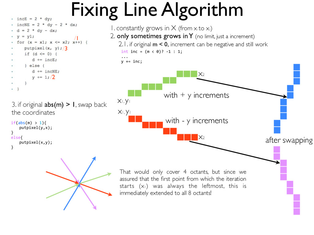
to x2 ) 2. only sometimes grows in Y (no limit, just a increment) 2.1. if original m < 0, increment can be negative and still work x2 x1, y1 /1 /2 x2 x1, y1 with + y increments with - y increments 3. if original abs(m) > 1, swap back the coordinates /3 if(abs(m) > 1){ putpixel(y,x); } else{ putpixel(x,y); } int inc = (m < 0)? -‐1 : 1; ... y += inc; after swapping That would only cover 4 octants, but since we assured that the first point from which the iteration starts (x1 ) was always the leftmost, this is immediately extended to all 8 octants!
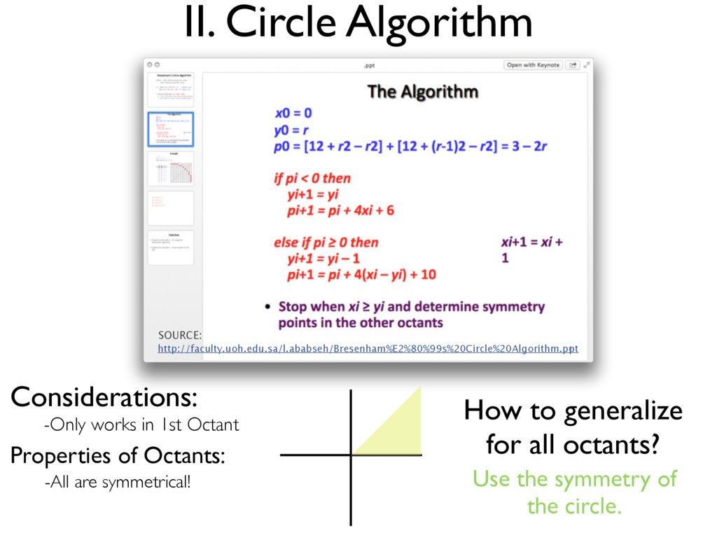
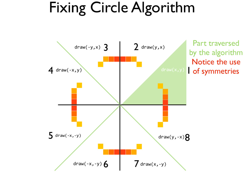
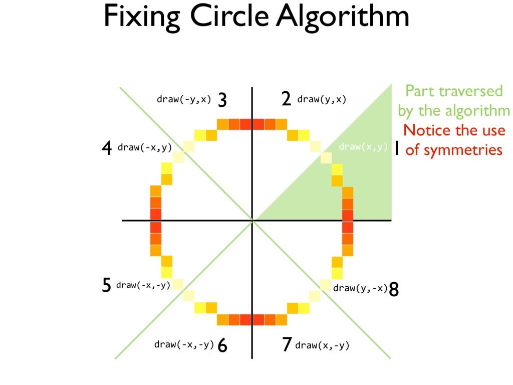
of Octants: -All are symmetrical! How to generalize for all octants? Use the symmetry of the circle. http://faculty.uoh.edu.sa/l.ababseh/Bresenham%E2%80%99s%20Circle%20Algorithm.ppt SOURCE:
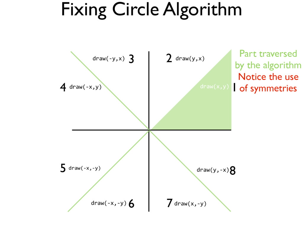
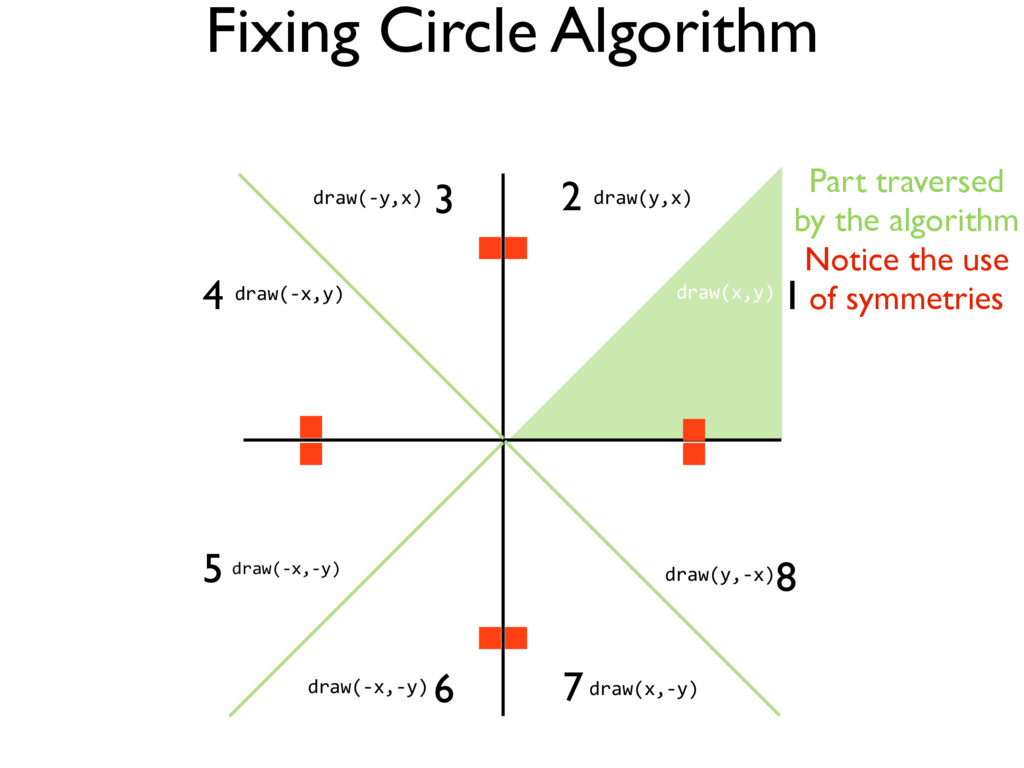
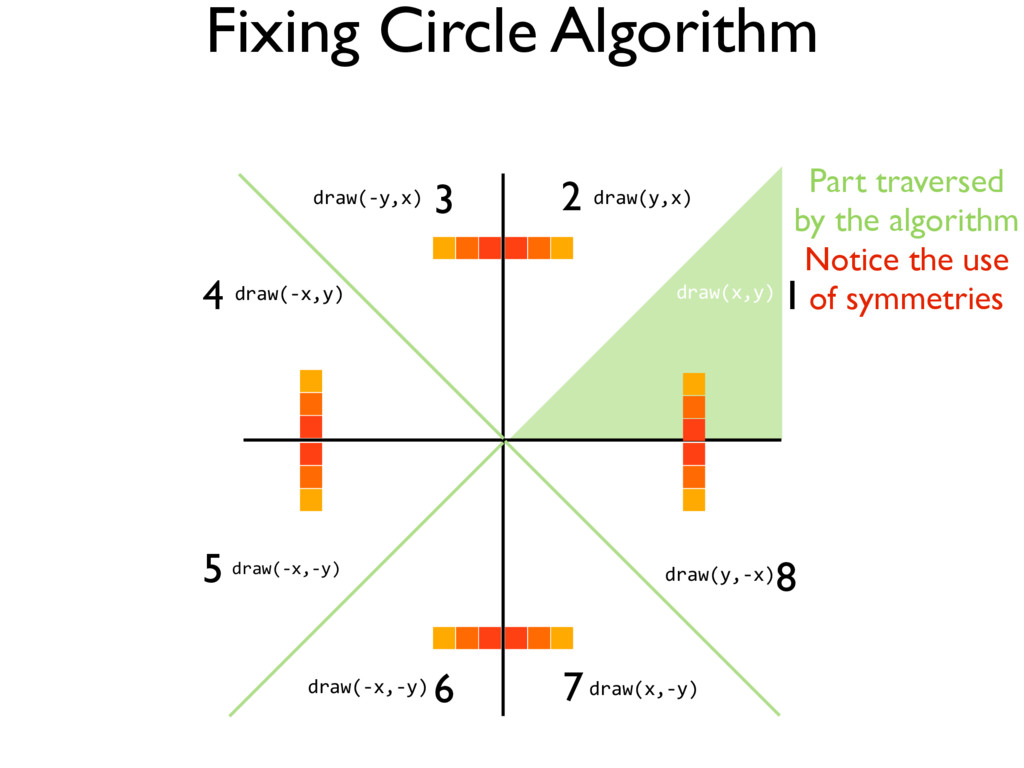
traversed by the algorithm Notice the use of symmetries draw(x,y) draw(y,x) draw(-‐y,x) draw(-‐x,y) draw(-‐x,-‐y) draw(-‐x,-‐y) 7draw(x,-‐y) 8 draw(y,-‐x)
traversed by the algorithm Notice the use of symmetries draw(x,y) draw(y,x) draw(-‐y,x) draw(-‐x,y) draw(-‐x,-‐y) draw(-‐x,-‐y) 7draw(x,-‐y) 8 draw(y,-‐x)
traversed by the algorithm Notice the use of symmetries draw(x,y) draw(y,x) draw(-‐y,x) draw(-‐x,y) draw(-‐x,-‐y) draw(-‐x,-‐y) 7draw(x,-‐y) 8 draw(y,-‐x)
traversed by the algorithm Notice the use of symmetries draw(x,y) draw(y,x) draw(-‐y,x) draw(-‐x,y) draw(-‐x,-‐y) draw(-‐x,-‐y) 7draw(x,-‐y) 8 draw(y,-‐x)
traversed by the algorithm Notice the use of symmetries draw(x,y) draw(y,x) draw(-‐y,x) draw(-‐x,y) draw(-‐x,-‐y) draw(-‐x,-‐y) 7draw(x,-‐y) 8 draw(y,-‐x)
traversed by the algorithm Notice the use of symmetries draw(x,y) draw(y,x) draw(-‐y,x) draw(-‐x,y) draw(-‐x,-‐y) draw(-‐x,-‐y) 7draw(x,-‐y) 8 draw(y,-‐x)
traversed by the algorithm Notice the use of symmetries draw(x,y) draw(y,x) draw(-‐y,x) draw(-‐x,y) draw(-‐x,-‐y) draw(-‐x,-‐y) 7draw(x,-‐y) 8 draw(y,-‐x)
which are cheap operations while inside the loop. • The control values which involve multiplication are computed only once, outside the loop, so their cost is almost meaningless. • Control values use only integers, which are fast for operations and doesn’t have the error induced by the use of floating point numbers.
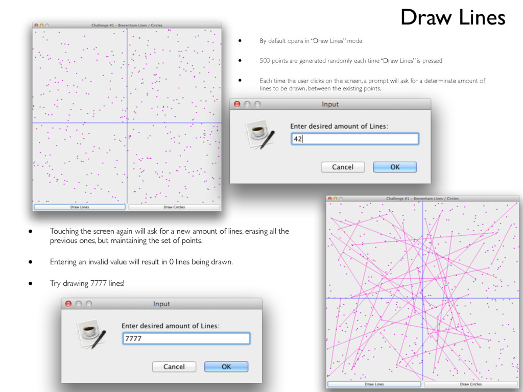
points are generated randomly each time “Draw Lines” is pressed • Each time the user clicks on the screen, a prompt will ask for a determinate amount of lines to be drawn, between the existing points. • Touching the screen again will ask for a new amount of lines, erasing all the previous ones, but maintaining the set of points. • Entering an invalid value will result in 0 lines being drawn. • Try drawing 7777 lines! Draw Lines
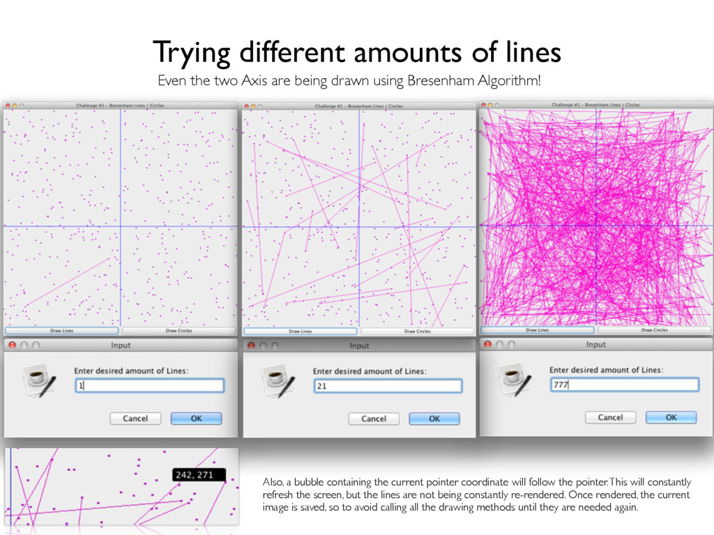
being drawn using Bresenham Algorithm! Also, a bubble containing the current pointer coordinate will follow the pointer. This will constantly refresh the screen, but the lines are not being constantly re-rendered. Once rendered, the current image is saved, so to avoid calling all the drawing methods until they are needed again.
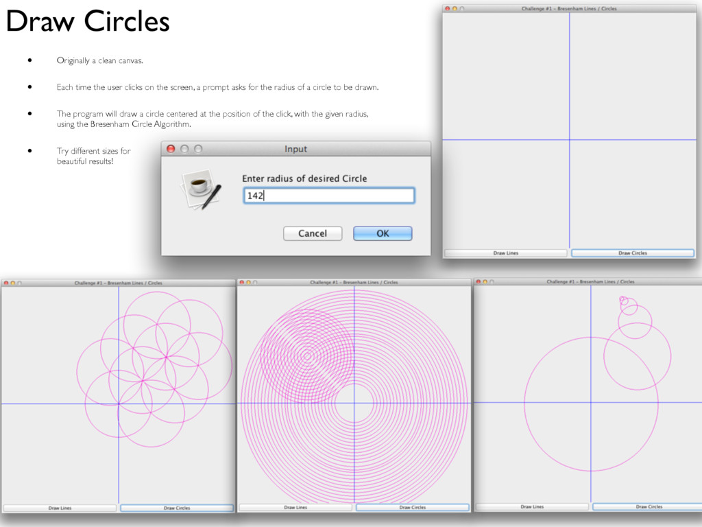
the user clicks on the screen, a prompt asks for the radius of a circle to be drawn. • The program will draw a circle centered at the position of the click, with the given radius, using the Bresenham Circle Algorithm. • Try different sizes for beautiful results!