Upgrade to Pro — share decks privately, control downloads, hide ads and more …

Exo-Obs Course: Spectroscopy and Radial Velocit...

Avatar for Adina Adina
September 28, 2025

Exo-Obs Course: Spectroscopy and Radial Velocity Technique

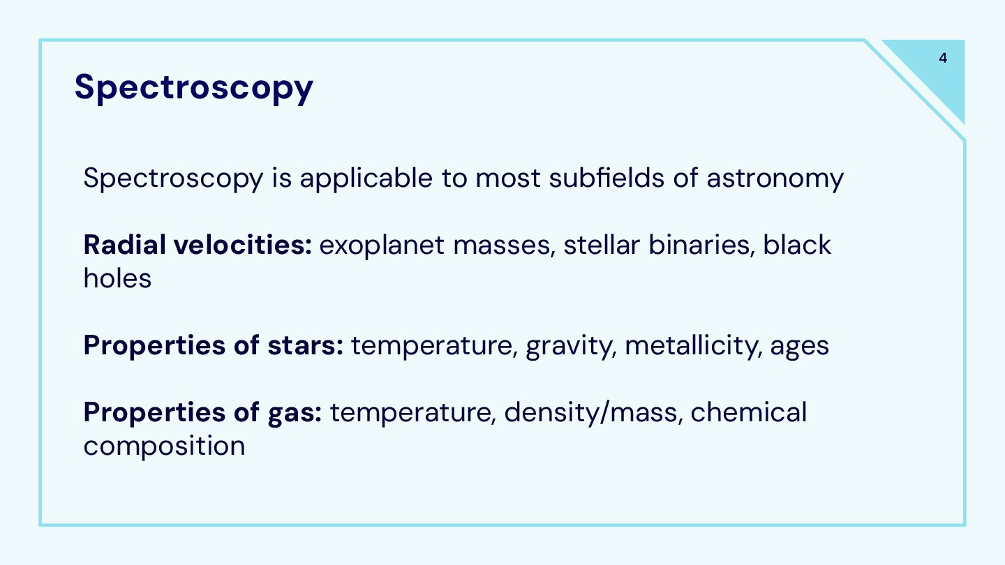
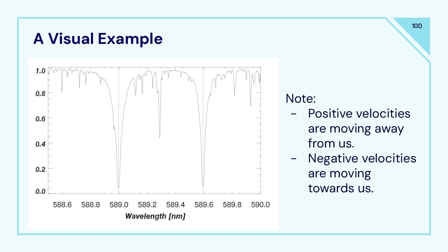
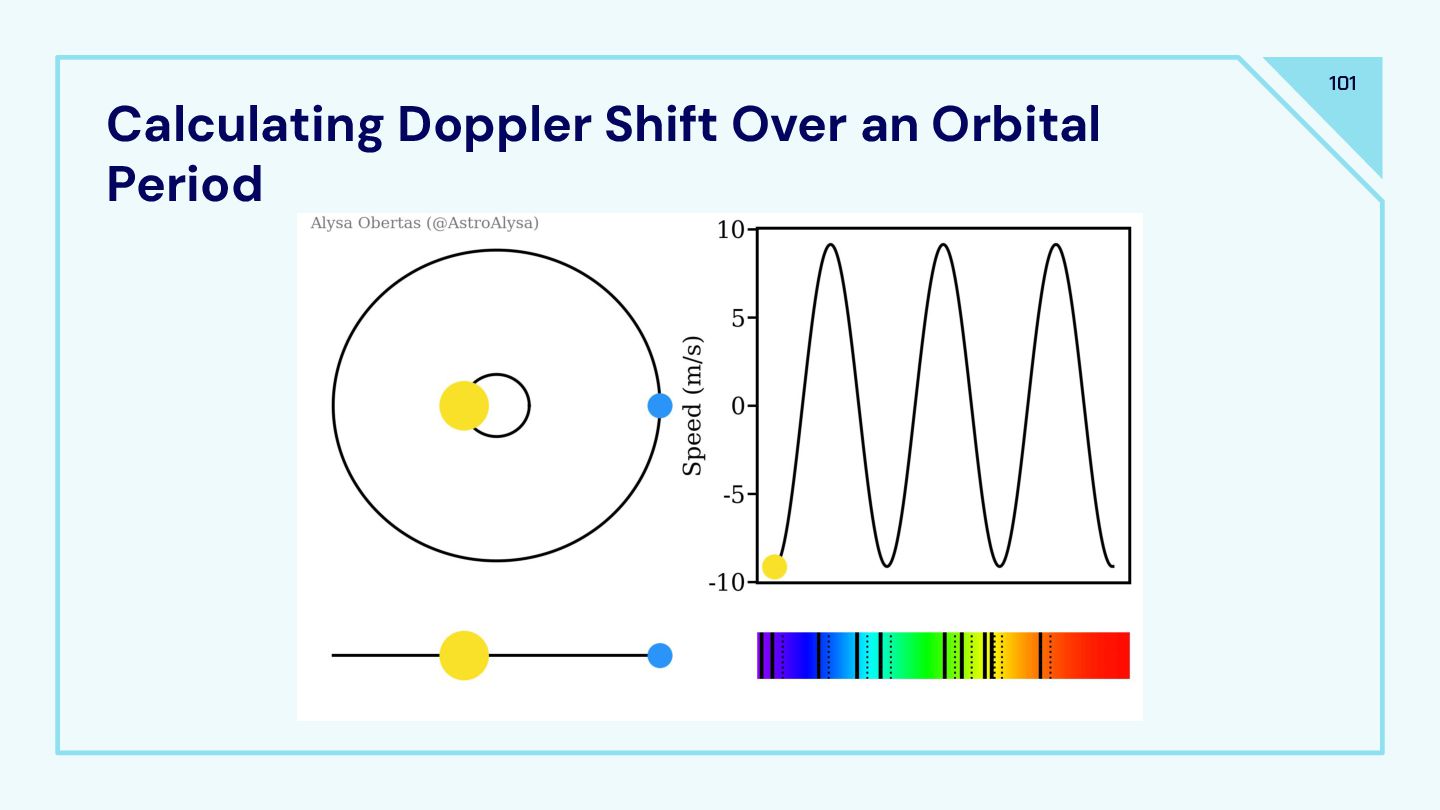
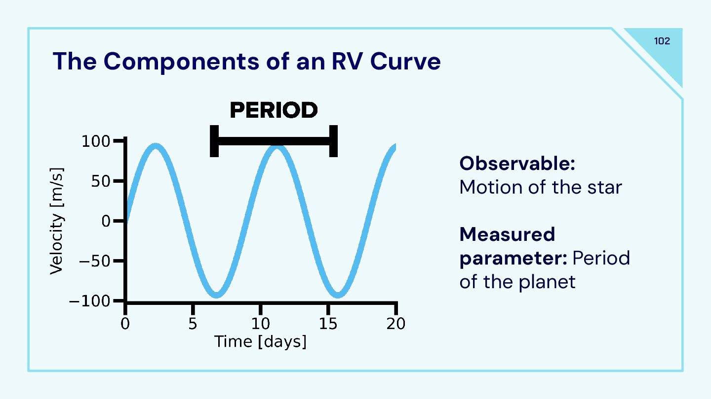
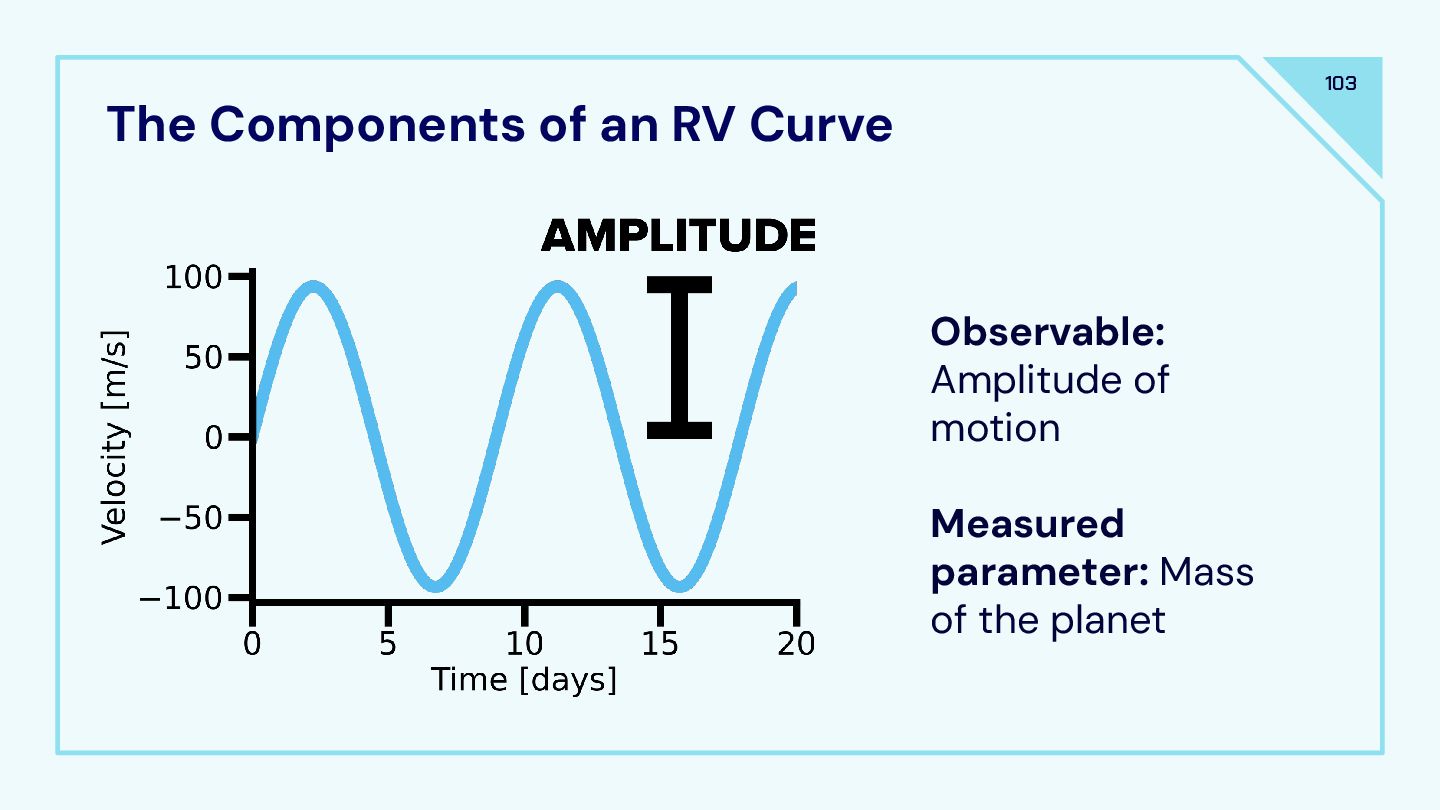
I will be sharing the slides I developed for a graduate level course on Exoplanets and Observational Astronomy. This is the second completed slide deck for this course. It covers topics on fundamentals of spectroscopy and radial velocity measurements for exoplanets.

Avatar for Adina

Adina

September 28, 2025
Tweet

More Decks by Adina

Other Decks in Science

Transcript

  1. Spectroscopy 4 Spectroscopy is applicable to most subfields of astronomy

    Radial velocities: exoplanet masses, stellar binaries, black holes Properties of stars: temperature, gravity, metallicity, ages Properties of gas: temperature, density/mass, chemical composition
  2. Spectral Resolution 5 The single most important number in spectroscopy

    is resolution R = λ/Δλ Δλ is interpreted as the closest spacing of lines that can be resolved. In practice, it is measured as the full width at half maximum (FWHM) of unresolved lines in the spectrum. Can be presented in wavelength [e.g., nm] or velocity [e.g., km/s].
  3. Spectral Resolution 6 Instrument resolutions typically range from R ~

    100 - 100,000. Different resolutions can achieve different scientific goals: • Low resolution: rough classification/redshift • Moderate resolution: basic stellar parameters, radial velocities of faint stars • High resolution: precise velocities and abundances, ideal for measuring masses of exoplanets Any of these resolutions are sufficient for looking at exoplanet atmospheres.
  4. Diffraction Limit 9 The scattering process is dependent on the

    wavelength and the size of the aperture: θ L = 1.22 λ / D Where D L is the diffraction limit, λ is the wavelength of light, and D is the diameter of the telescope. Mathematically, the limit is defined as where the first ring occurs.
  5. Slits & Slitmasks 11 Dispersing the entire sky would add

    noise to a target spectrum. Plus, all of the stellar spectra would overlap. Slitless spectroscopy is a thing. Simulated dispersed spectra from JWST/NIRCam.
  6. Slit Width 12 An instrument’s resolution is set by the

    slit and the grating. In principle, the slit can be narrowed to the diffraction limit. Real slits must be wide enough to pass much/most of the light from the typical seeing. One way to get a higher resolution spectrum is to use a smaller slit. Wider slits may also be used to observe more extended objects (e.g., galaxies).
  7. Collimator 14 The beam from the primary mirror is converging.

    The light is arriving at different angles. The collimator aligns the rays of light to be parallel before it reaches the grating.
  8. Gratings: Constructive Interference 17 You get constructive interference if the

    path length between rays from neighboring slits is an integer multiple of the wavelength. d sinθ = m λ (for m = 0, +/-1, +/-2…)
  9. Gratings: Destructive Interference 18 You get destructive interference if the

    wavelength is ½ different from the path length. d sinθ = (m + ½) λ
  10. Gratings: Slit Locations 19 Adding new slits with the same

    spacing does not change the locations of constructive interference d sinθ = m λ However, it does make those peaks brighter. On the contrary, adding new slits does change the locations of destructive interference, moving them closer to the constructive peaks.
  11. Gratings: Slit Locations 21 To get a spectrum, you put

    a CCD at one of the constructive peaks. You can see that it’s already more complicated than that, as rainbows disperse and overlap.
  12. Gratings: Spectral Overlap 22 The rainbows overlap at sin θ

    1 = m λ/d = (2m)(λ/2)/d To first order, a spectrum at 8000Å would have second-order light at 4000Å. The orders must be sorted (either rejected via a filter or cross-dispersed).
  13. Gratings: Cross-Dispersion 23 Single slit spectroscopy puts a filter over

    the grating to sort-out the specific wavelengths someone wants. A cross-dispersed spectrograph spreads the light across the detector into orders.
  14. Gratings: Estimating Resolution 24 We estimate the resolution of a

    grating by equating the nearest destructive peak at one wavelength to the constructive peak of the nearest “resolved” wavelength sin(θ+Δθ) = (m + 1/N)λ/d = m(λ+Δλ)/d λ/Δλ = mN The resolution only depends on the total number of slits.
  15. Gratings: Improving Resolution 25 1. Go to higher order a.

    Requires cross-dispersion to avoid overlap 2. Use a finer spacing of slits a. Physical limits to spacing (~1200 slits/lines per mm) is the finest we can realistically go 3. Make a larger grating a. Limited by the size of the delivered beam
  16. Gratings: Improving Resolution 26 1. Go to higher order a.

    Requires cross-dispersion to avoid overlap 2. Use a finer spacing of slits a. Physical limits to spacing (~1200 slits/lines per mm) is the finest we can realistically go 3. Make a larger grating a. Limited by the size of the delivered beam
  17. Reflection Gratings 27 One issue with transmission gratings is that

    the highest power is put into the useless m=0 order with no dispersion (perpendicular to the detector. By replacing the grid of slits with a “sawtooth” grating, we can increase the power at higher orders (m >= 1).
  18. Reflection Gratings 28 Reflection gratings obey a more complicated equation:

    d (sinα + sinβ) = m λ The “Littrow” condition is the highest efficiency, when these angles are equal. Gratings are typically blazed close to this condition
  19. VPH Grating 30 Many newer instruments use volume phase holographic

    (VPH) gratings. VPH gratings use laser-imprinted modulations in the index of refraction in a gelatinous material to design the interference pattern. They are operated at the Littrow condition, so they provide a higher efficiency and transmission and allow for a more compact instrument.
  20. Camera 32 After the light is dispersed, it needs to

    be refocused to be an imaged. In its most basic form, a spectrograph produces images of the slit with the wavelengths spread out.
  21. Plate Scale 33 p = θ/s = 206265”/(D · f-ratio)

    [pixels] D is the diameter of the telescope [length] f-ratio is the ratio of the focal length to the diameter [unitless] f-ratio = F / D
  22. What is the plate scale if you use a 1”

    slit on SOAR (D = 4.1m; f-ratio = 16.6)? 34
  23. Plate Scale 35 The spectrograph demagnifies the image by a

    the factor f cam /f coll If we assume the collimator is not powered, we need a factor of 8-10 demagnification at the camera to get a normal ~2-3 pixel slit. To achieve this, the camera has to be fast (f/1.7 - f/2.0). Faster cameras are bigger and more expensive.
  24. Multi-Object Spectroscopy 36 Some spectrographs offer pre-fabricated masks covering multiple

    objects of interest. Pros: multiple objects at once, good sky subtraction Cons: object selection is limited by spatial conflicts, spectral coverage varies by position, complicated to design, not flexible
  25. Multi-Object Spectroscopy 37 Designing the slits: 1. Prefabricated physical masks

    + fiber-fed spectroscopy (e.g., SDSS plates). This design runs optical fibers from the focal planet to the instrument. 2. Micro-electro-mechanical shutters (MEMS). This design uses a programmable grid of millions of tiny shutters. Currently being used by JWST/NIRSpec.
  26. Multi-Object Spectroscopy: ADC 38 Multi-object spectrographs commonly used atmospheric dispersion

    correctors (ADC). ADCs have pairs of prisms that can correct for dispersion as a function of sky position. ADCs are useful for multi-object spectrographs, when the slit angle cannot be arbitrarily set.
  27. Integral Field Unit (IFU) 39 Offers spectra at each position

    in a 2D image. Typically have small FOV and are used with AO imaging.
  28. 48 Spatial Profile The spatial profile is a vertical slice

    along the detector, including the object in the slit. An example is shown here → Discussion: What sets the spatial profile of a given object?
  29. Spatial Profile 49 What sets the spatial profile? 1. The

    object itself. A point source (e.g., star) is dominated by the seeing PSF while an extended source (e.g., galaxy) is dominated by the object’s surface brightness distribution. 2. Seeing. Seeing spreads the object’s light into a ~Gaussian PSF. 3. Slit width. If the slit is wider than the seeing disk, the profile will look like the PSF. If the slit is narrower, it will have a boxy profile. 4. Optics. Slit function, detector sampling, etc.
  30. Arc Lamp 52 Arc lamps allow you to map the

    pixel location to a wavelength. For most spectrographs, you need an arc lamp for every science target you observe. Why?
  31. Arc Lamp 53 Many spectrographs have one lamp to use.

    Sometimes, spectrographs have multiple lamps available to select from. The selection will depend on what wavelengths you are observing at.
  32. Sky Lines in the Red 54 If you are working

    in the red optical or infrared, you can sometimes use sky lines instead of an arc lamp.
  33. Flat Fields 55 Lamps are a poor match to the

    night sky, so flat fields can be taken for imaging to mitigate pixel-to-pixel differences on the detector.
  34. Flat Fields 57 Because it is difficult to map between

    pixel and wavelength, it is hard to ensure that removing the pixel variations is helping the S/N, rather than hurting it.
  35. Telluric Standard 58 When observing in the far red/near-infrared, it

    is common to observe a telluric standard (A star) to remove the effect of sky absorption lines.
  36. Atmospheric Refraction 60 Atmospheric refraction doesn’t matter as much for

    imaging, but it matters a lot for spectroscopy. We can minimize atmospheric refraction by observing at the parallactic angle. For the parallactic angle, we align the dispersion to always be perpendicular to the horizon. This results in the relative angle between the dispersion and a fixed direction changes with time.
  37. Atmospheric Refraction 61 If you do not observe at the

    parallactic angle, you will lose sensitivity out at bluer wavelengths!
  38. Things you need to consider when planning your observations 63

    1. Grating - determines your resolution and wavelength coverage
  39. Things you need to consider when planning your observations 65

    1. Grating - determines your resolution and wavelength coverage 2. Slit width - usually set by seeing and your object type
  40. Slit width Selection 66 Slit width selection will be dependent

    on your source and seeing. Slit losses increase quickly as you go to worse seeing. The optical slit is ~(4/3) * FWHM You can use smaller slits to get higher S/N and higher resolution spectra (especially for stars).
  41. Things you need to consider when planning your observations 67

    1. Grating - determines your resolution and wavelength coverage 2. Slit width - usually set by seeing and your object type 3. Binning - want a wide enough FWHM in both the spatial and spectral directions
  42. Binning Selection 68 For spatial binning, you want 2+ pixels

    FWHM for accurate centering. Anything smaller than 2-pixels could be lost to read noise. For spectral binning, you want arguably 3+ pixels FWHM because you are more interested in fitting the line profiles (e.g., for broadened lines). I typically do not bin spectral when looking at stars.
  43. Things you need to consider when planning your observations 69

    1. Grating - determines your resolution and wavelength coverage 2. Slit width - usually set by seeing and your object type 3. Binning - want a wide enough FWHM in both the spatial and spectral directions 4. Read noise/gain - typically want the lowest/slowest read noise for spectra
  44. Readout Rate Example: SOAR/GODMAN 70 Read Rate [kHz] Analog ATTN

    Gain [e-/ADU] Read Noise [e-] 50% Full Well [ADU] 100 3 1.54 3.45 66,558 100 2 3.48 5.88 29,454 344 3 1.48 3.89 69,257 344 0 3.87 7.05 26,486 750 2 1.47 5.27 69,728 750 0 3.77 8.99 27,188
  45. Things you need to consider when planning your observations 71

    1. Grating - determines your resolution and wavelength coverage 2. Slit width - usually set by seeing and your object type 3. Binning - want a wide enough FWHM in both the spatial and spectral directions 4. Read noise/gain - typically want the lowest/slowest read noise for spectra 5. Calibration lamp - essential for wavelength calibration
  46. Selecting Calibration Lamps 72 You want to make sure that

    you select a lamp that has a sufficient number of lines in the wavelength range you are interested in. https://soardocs.readthedocs.io/projects/lamps/en/latest/ Make sure you check your arcs when you take them!
  47. Observing Ordering 73 1. Take a spectrum of your source

    2. Take a calibration lamp* 3. For NIR spectroscopy - take a spectrum of a standard star 4. For NIR spectroscopy - take a calibration lamp for the standard 5. Rinse and repeat * You should take your lamp immediately after your science spectrum because the location of the spectrum could shift when the telescope moves.
  48. Step 2: Subtract overscan 76 Subtract an average along each

    row or take an average along the columns, then fit a function to the rows and subtract (IRAF routine: ccdproc)
  49. Step 3: Trim 77 Remove the regions of the image

    where there the chip is unilluminated (IRAF routine: ccdproc)
  50. Step 4: Remove cosmic rays 78 There are lots of

    routines to do this for you, so you don’t have to reinvent the wheel. The most common routine is L.A. Cosmic (https://lacosmic.readthedocs.io/en/stable/)
  51. (Optional) Step 6: Flat fielding 80 For high-resolution spectroscopy, you

    may want to subtract your flat field images. For low-resolution spectroscopy, this may introduce more noise than it is worth.
  52. Step 7: Extract your spectrum 81 a. Select the extraction

    aperture size b. Find the object c. Trace the location of the object in each column d. Subtract the background IRAF: apall function
  53. Step 7a: Selecting your aperture 82 The ideal aperture has

    ~90% of the light from the star. The remaining 10% is “too expensive” to get, meaning it’s not worth the trade-off of introducing noise from the background. It is okay to experiment with different apertures for each data set. You can compare differences in the continuum, absorption features, and sky lines to empirically derive a “best” aperture.
  54. Step 7a: Selecting your aperture 83 In reality, a lot

    of people use the “optimal extraction” method, which weighs brighter pixels more. This is the equivalent to PSF fitting. The O.G. optimal extraction algorithm publication: Horne (1986).
  55. Step 7b: Identifying the object 84 Select a region around

    (~10-25 pixels) where the trace appears to be. Fit a profile (typically Gaussian) to the column. The peak in the Gaussian is roughly where the source is.
  56. Step 7c: Identifying the trace 85 Repeat this process in

    each column as the trace may be curved. Once you have a position of the trace in each column, you should fit trace location with a high-order polynomial (4th order is typically good).
  57. Step 7c: Identifying the trace (aside) 86 The amount of

    curvature will be dependent on the optical distortion of the camera and dispersion geometry.
  58. Step 7d: Removing the background 87 Background subtraction is done

    on a column-by-column basis. There are many ways to handle background subtraction. For long-slit spectroscopy, you may want to take an average of a small region around where the object is and subtract that from the column.
  59. Step 7d: Removing the background (aside) 88 This won’t work

    for extended sources. You will need to rectify (straighten) the sky lines first before removing the background.
  60. Step 8: Wavelength calibration (the hardest part) 89 Extract the

    arc spectrum using the same trace identified in the science frame. Do not do any background subtraction.
  61. Step 8: Wavelength calibration (the hardest part) 90 You will

    have to identify a handful of emission lines (by-eye, most likely). Make sure you identify lines across the entire spectrum, otherwise your calibration may be off. Lines can be identified using a standard “line list.”
  62. Step 8: Wavelength calibration (the hardest part) 91 You will

    fit the relationship between wavelength (x-axis) and pixel location (y-axis). Use the lowest order fit possible. You can check how the order fit looks by calculating the RMS of the residuals.
  63. Step 8: Wavelength calibration (the hardest part) 92 Check the

    residuals of your fit. Trim any outliers you may have and re-fit. This will be an iterative process. (IRAF: identify)
  64. Step 8: Wavelength calibration (the hardest part) 93 The best

    course of action is using a recent calibration from someone else for a similar setup (why reinvent the wheel). The second best approach is to use an identified list/image on the instrument website, although the relative line strengths usually vary between lamps and over time. Most often, you will create your own wavelength solution for each spectrum you have.
  65. Step 8: Wavelength calibration (the hardest part) 94 A typically

    good fit to low-resolution spectroscopy has a precision of 0.05-0.1 Å (3-6 km/s) rms. You can achieve ~5+ better at moderate resolution. A lot of reductions are done by feel (a.k.a. The o.g. neural network). Once you know an instrument well enough and have done enough reductions, you will feel out what a good RMS should be.
  66. Step 9: Applying the wavelength solution 95 The wavelength solution

    is typically nonlinear. While you could look at a spectrum with a non-linear wavelength solution, it is harder to do science with (e.g., take fourier transforms). To linearize your spectrum, you must rebin the pixels such that the spectral dispersion is constant in either linear (every pixel = constant # of Å) or log-linear (every pixel = constant # of log(Å)) space.
  67. Step 9: Applying the wavelength solution 96 To do this,

    you must interpolate your spectrum. This is why we need a well-sampled FWHM in the spectral direction. This does result in correlated adjacent pixel noise, but it’s fine for most science cases.
  68. Correcting for the Earth 97 When we care about measuring

    radial velocities, we need to correct velocities that are caused by the Earth. The Earth orbits the solar system barycenter at ~30 km/s. At the same time, the Earth rotates at ~0.5 km/s. All of these velocities must be corrected to get precise radial velocity measurements. https://astroutils.astronomy.osu.edu/exofast/barycorr.html
  69. The Concept 99 Radial velocity measurements rely on the doppler

    effect. ∆λ v star λ 0 c Where: λ 0 is the wavelength of the absorption line in the rest frame. ∆λ is the measured shift in wavelength from λ 0 . v star is the velocity. c is the speed of light. =
  70. A Visual Example 100 Note: - Positive velocities are moving

    away from us. - Negative velocities are moving towards us.
  71. The Components of an RV Curve 102 Observable: Motion of

    the star Measured parameter: Period of the planet
  72. The Components of an RV Curve 103 Observable: Amplitude of

    motion Measured parameter: Mass of the planet
  73. Deriving Orbital and Planetary Properties from the Radial Velocity Curve

    104 Assuming a circular orbit, the velocity of the planet, v p , and the velocity of the star, v ⭑ , are expressed as Real orbits aren’t necessarily aligned with our line of sight. To account for a projection effect, we introduce an inclination term where
  74. Deriving Orbital and Planetary Properties from the Radial Velocity Curve

    105 Taking the ratio of the velocities, we find that From the definition of the center of mass (M p r p = M ⭑ r ⭑ ), we can write this
  75. Deriving Orbital and Planetary Properties from the Radial Velocity Curve

    106 Kepler’s 3rd Law: Planet Semi-major axis, a Sun Orbital period, P M tot = M p + M ⭑ The semi-major axis is related to r p and r ⭑ as
  76. Deriving Orbital and Planetary Properties from the Radial Velocity Curve

    107 The radial velocity semi-amplitude, K ≡ v ⭑, obs . From all of the previously discussed equations, derive K.
  77. Deriving Orbital and Planetary Properties from the Radial Velocity Curve

    108 The radial velocity semi-amplitude, K ≡ v ⭑, obs . From all of the previously discussed equations, derive K.
  78. THE radial velocity calculation 109 K = semi-amplitude of the

    radial velocity curve P = period M p = mass of planet M star = mass of the central star e = eccentricity i = inclination
  79. The Components of an RV Curve 110 Observable: shape of

    the RV curve Measured parameter: eccentricity of the orbit
  80. Guesstimating Masses 111 Planetary Mass [M ⊕ ] Radial Velocity

    Signal @ 1 AU [m s-1] 1 0.09 16 1.5 320 28
  81. Guesstimating Masses 112 Planetary Mass [M ⊕ ] Radial Velocity

    Signal @ 1 AU [m s-1] 1 0.09 16 1.5 320 28
  82. Guesstimating Masses 113 Planetary Mass [M ⊕ ] Radial Velocity

    Signal @ 1 AU [m s-1] 1 0.09 16 1.5 320 28
  83. Guesstimating Masses 114 Planetary Mass [M ⊕ ] Radial Velocity

    Signal @ 1 AU [m s-1] 1 0.09 16 1.5 320 28
  84. Rossiter-McLaughlin Effect 116 The spin-orbit alignment (obliquity) is the angle

    between the stellar spin axis and the planet’s orbital plane. In theory, it may be able to tell you about the formation history of a given system.
  85. Rossiter-McLaughlin Effect 118 As a planet transits its star, it

    temporarily blocks part of the blue-shifted and red-shifted hemispheres, making the star appear redder or bluer. By looking at how the RVs change across a given transit, you can better understand the orientation of the orbital plane.
  86. Doppler Tomography 119 Doppler tomography is another analysis technique to

    measure the spin-orbit alignment of a system. Instead of calculating the RVs, you can measure the small deviations in a line profile as a planet transits the blue-shifted and red-shifted limbs of the star. Requires high resolution spectra.
  87. DISCUSSION QUESTION All stars are good stars, but some stars

    are better for RVs. Which spectral type do you think are the best for blind RV searches? 125
  88. Spectral Type Dependence 126 OBA • Too few absorption lines

    • Fast rotating (even on the main sequence) • Short-lived FGKM • Sufficient lines • Slower rotators (most times) • Solar-like stars have M star = 0.7 - 1.3 M ⊙ Created by: David Wilson
  89. Rotational Line Broadening 128 Red light is slightly redshifted Blue

    light is slightly blueshifted wavelength intensity
  90. wavelength intensity wavelength intensity Rotational Line Broadening 129 Red light

    is slightly redshifted Blue light is slightly blueshifted Red light is slightly redshifted Blue light is slightly blueshifted
  91. Stellar “Jitter” a.k.a. Physics 130 What exoplanet astronomers think stars

    look like What stars actually look like (probably)
  92. Oscillations 131 Stars aren’t in perfect hydrostatic equilibrium (gravity balanced

    by internal pressure). Small perturbations from equilibrium causes the stellar plasma to expand or compress, generating waves.
  93. Oscillations: p-modes 132 Pressure Modes (p-modes) ~ sound waves inside

    the star. The frequency of p-modes depends on the internal temperature and structure of the star (asteroseismology). For solar-like stars, p-modes are driven by stochastic convection on the stellar surface.
  94. Oscillations: p-modes 133 The spacing between consecutive overtones is given

    by Δ𝜈 = √⍴ Where 𝜈 = frequency and ⍴ is the stellar density. l are the acoustic modes
  95. Oscillations: p-modes 134 With just measuring the spacing between frequencies

    and knowing the temperature of the star, you can derive precise fundamental stellar parameters: Kjeldsen & Bedding (1995)
  96. Oscillations: g-modes 136 Gravity Modes (g-modes) - driven by the

    motion of plasma turbules in the deep interior of stars. G-modes are often significantly dampened when they reach the surface, so they are hard to detect, but a powerful tool.
  97. Granulation 137 The motion of convective cells on the photosphere.

    Granules have typical scale lengths of ~1000 km and velocities of ~1 km/s. Bright = upward motion of hot gas Dark = downward motion of cool gas Timescale: ~10s of minutes
  98. Starspots 138 Sunspots form when tangled magnetic field lines rise

    to the Sun’s surface. Lines are twisted by the Sun’s differential rotation (the equator spins faster than the poles). The field lines inhibit the flow of heat from the interior, making cooler (darker) regions.
  99. Activity Cycles 140 Every 11-years, the magnetic field on the

    Sun flips polarity (north → south; south → north). It is driven by the solar dynamo (the physical process that generates the magnetic field).
  100. Activity Indicators 143 There has been a lot of work

    trying to use lines that trace magnetic activity to remove stellar-related activity from radial velocity measurements. Lafarga et al. (2023) de Beurs et al. (2022)