Upgrade to Pro — share decks privately, control downloads, hide ads and more …

Exo-Obs Course: Key Observational Concepts, AO,...

Avatar for Adina Adina
November 09, 2025

Exo-Obs Course: Key Observational Concepts, AO, and Direct Imaging

I will be sharing the slides I developed for a graduate level course on Exoplanets and Observational Astronomy. This is the fourth completed slide deck for this course. It covers topics on fundamentals of time, ground-based observing limitations, adaptive optics imaging, and directly imaged exoplanets.

The photometry slides were adapted from Jay Strader's graduate course elective on observational astronomy.
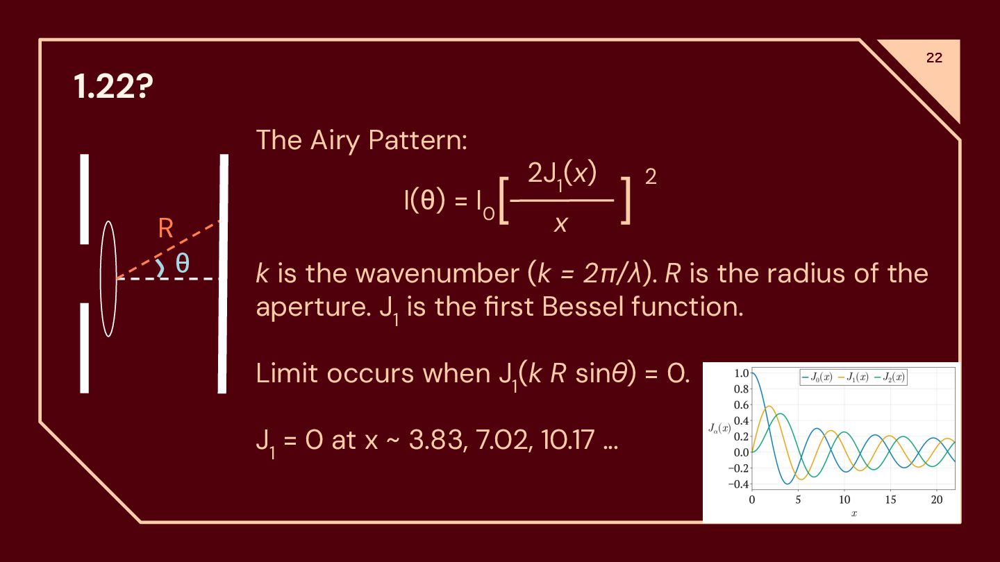
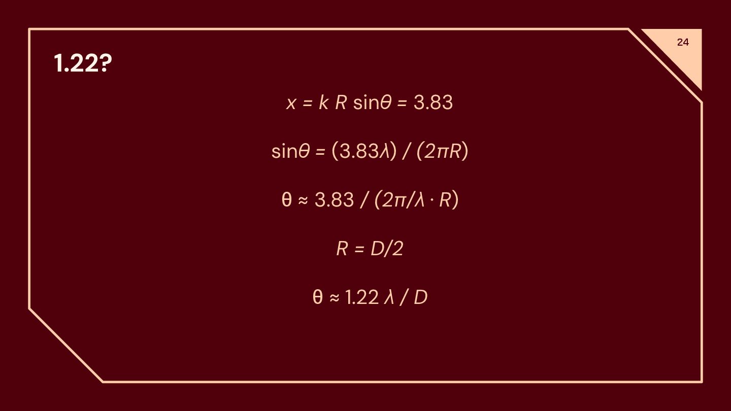
Avatar for Adina

Adina

November 09, 2025
Tweet

More Decks by Adina

Other Decks in Science

Transcript

  1. Time* has many purposes • Keep precise count of seconds

    for specific/technical reasons • Track our everyday existence on Earth These goals are inconsistent. And so, we created one million different systems to keep track of time for different purposes. * Time is a social construct. 4
  2. Day to Day Time (Sun time) The simplest definition of

    “noon” is when the Sun crosses the local meridian (i.e. when the Sun is highest in the sky). Sun-time varies by +/- 15 minutes depending on the time of the year. Affected by Earth’s obliquity + eccentricity. 5
  3. Greenwich Mean Time Mean solar time in Greenwich, London. Arose

    after the adoption of clocks as a means of navigation (for longitude) on naval ships. Invention of railroads required standard time, where noon had to mean the same thing in different places. And thus, the time zone system was born. 6
  4. Universal Time (UT1) Modern time standard based on Earth’s rotation.

    Mean solar time at longitude = 0. It is an idealized modern version of GMT time. Atomic Time (TAI) “Fundamental” time from atomic clocks. They are accurate to 1 part in 1016, It is the weighted average of 400 atomic clocks with appropriate general relativistic corrections. 8 These systems do not stay in sync due to Earth’s rotation, which slows by 1.4ms per day due to tidal forces from the Moon.. This is an acceptable reason to hate the Moon.
  5. Coordinated Universal Time (UTC) 9 UTC is kept within 0.9

    s of TAI by adding leap seconds every couple of years Currently: TAI - UTC = 37s UTC is a reasonable compromise. Typically, when astronomers use a date and don’t give units, it’s in UTC.
  6. Julian Date (JD) 10 Numbers are easier to parse than

    weird strings. T0 = January 1, 4713 BCE Note that the Julian calendar is 5 weeks earlier in the Gregorian calendar
  7. Modified Julian Date (MJD) 11 Computers used to have low

    memory MJD = JD - 2400000.5 Basically, it just drops the first two digits and makes the day start at midnight, rather than noon
  8. Modified Julian Date (MJD) 13 JD/MJD do not take the

    Earth’s movement into account. This is one reason why a transit or eclipse can be shifted by +/- 500 s, depending on where the Earth is Correcting for the Sun gives us “heliocentric julian date” (HJD)*, which is better, but not ideal. * I have only seen HJD used in the JWST Astronomer’s Proposal Tool. It’s only a few seconds different from MJD.
  9. Barycentric Julian Date (BJD) 14 The ideal time units. BJD

    uses atomic time and corrects it to the solar system barycenter and for general relativity effects. BJD should always be used for exoplanet studies!
  10. Jay’s Formula for Success 15 1. Get the midpoint of

    your exposure in UTC 2. Check that the time makes sense 3. Convert to BJD 4. Write a good paper 5. Get famous
  11. Sidereal Time 16 Sidereal day = real rotation period of

    Earth. Earth’s rotation period is 23h 56m 04s. We add an extra 4 minutes to account for the movement of the Sun. Sidereal time is nearly equivalent to UT1
  12. Sidereal Time 17 Sidereal time is a star clock. We

    use sidereal time to track objects that do not have fast apparent motion in the sky (e.g., exoplanets, stars, galaxies). The local sidereal time is the right ascension currently crossing your meridian. Sidereal time is relative to a specific location. We use non-sidereal tracking to observe objects with fast apparent motion in the sky (e.g., comets, alien spacecrafts).
  13. Determining What’s Observable When 18 We can measure a star’s

    longitude (R.A.) in degrees or hours, minutes, seconds. If a star with an R.A. of 6 hours is on the meridian, then we know that a star with an R.A. of 8 hours will be on the meridian in how many hours?
  14. Diffraction Limit 20 The diffraction limit is the highest angular

    resolution a telescope is able to achieve. When light hits an aperture, it bends and spreads, known as diffraction. Point sources, like stars, spread into a small disk with concentric rings (Airy Pattern).
  15. Diffraction Limit 21 The scattering process is dependent on the

    wavelength and the size of the aperture: θ L = 1.22 λ / D Where D L is the diffraction limit, λ is the wavelength of light, and D is the diameter of the telescope. Mathematically, the limit is defined as where the first ring occurs.
  16. 1.22? 22 The Airy Pattern: k is the wavenumber (k

    = 2π/λ). R is the radius of the aperture. J 1 is the first Bessel function. Limit occurs when J 1 (k R sinθ) = 0. J 1 = 0 at x ~ 3.83, 7.02, 10.17 … θ R [ ] 2 2J 1 (x) x I(θ) = I 0
  17. [ ] 2 1.22? 23 The Airy Pattern: • k

    = 2π/λ. • R is the radius of the aperture. • x = k R sinθ. • x = 3.83. Derive the Diffraction Limit. I(θ) = I 0 2J 1 (x) x
  18. 1.22? 24 x = k R sinθ = 3.83 sinθ

    = (3.83λ) / (2πR) θ ≈ 3.83 / (2π/λ · R) R = D/2 θ ≈ 1.22 λ / D
  19. Diffraction Limit 25 Working at the diffraction limit gets us

    finer imaging resolution. However, even at a very good site, you are typically limited to a resolution of a factor of ~25-50 worse due to seeing.
  20. Seeing 26 Seeing is used to collectively describe a variety

    of ways in which temperature variations in the atmosphere affect your images. Seeing is not your friend.
  21. Refraction Atmosphere 27 What happens to a light wave when

    it enters Earth’s atmosphere? Air has a refractive index of n~1.0003 at standard temperature and pressure (STP). Vacuum
  22. Refraction Atmosphere 28 To 0th order: (a) Light moves slower

    when it enters the atmosphere by v~ c/1.0003 (b) The wavelengths are shorter by λ ~ λ vacuum /1.0003 In reality, all of these factors depend on pressure, temperature, wavelength, and humidity. Vacuum
  23. Temperature Dependence of n 29 (n - 1) ~ ⍴

    δn ~ δ⍴/⍴ (n - 1) Consider two neighboring air blobs in the atmospheres. They will be in pressure equilibrium, so we can assume the ideal gas law P ∝⍴T = c 0
  24. Temperature Dependence of n 30 P ∝⍴T = c 0

    Implies Tδ⍴ + ⍴δT = 0 Combined with δn ~ δ⍴/⍴ (n - 1) You get δn~ δT/T (n - 1) Assuming n = 1.0003 and T = 210K (typical for the tropopause), a 1K change in temperature will correspond to light refracting by how many arcseconds?
  25. Turbulence 32 The tropopause is the boundary between the lower

    and upper atmosphere (troposphere -> tropopause -> stratosphere). The bulk of atmospheric turbulence exists in the tropopause. The tropopause is the start of an inversion layer, where temperature increases, rather than decreases, with height. Inversion layers are stable against turbulence.
  26. Bonus Slides: Quantifying Turbulence The sum of the scatterings produces

    a distorted wavefront. It is typical to summarize with r 0 , a length scale over which the root-mean-square (RMS) variation is 1 radian. You want a bigger r 0 . One can also think of this as the size of the telescope that would give the same diffraction-limited image as the seeing. Primary mirror of telescope Wavefront of light r 0 “Fried parameter” 33
  27. Bonus Slides: Quantifying Turbulence The classical turbulence model is a

    Kolmogorov spectrum: energy is fed in on large scales, then cascades to smaller scales. Kolmogorov model is a power law with a free parameter that is an integral over the turbulence profile. This model predicts r 0 ~ y (λ/5000Å)6/5(sec z)-⅗ y = 15-20cm. A good site like SOAR will have ~25 cm. An okay site might have 15-20 cm. r 0 changes nightly. 34
  28. Bonus Slides: Quantifying Turbulence r 0 ~ y (λ/5000Å)6/5(sec z)-⅗

    Since the seeing as a function of wavelength goes as λ/r 0 , we see that seeing ~ λ-⅕ This means that if the seeing isi 0.8’’ in V, it is expected to be 0.6’’ in K. Additionally, since Seeing ~ airmass3/5 We see that zenith seeing of ~0.8’’ implies 1.2’’ seeing at 2 airmasses: much worse! 35
  29. Bonus Slides: Quantifying Turbulence r 0 has a corresponding angular

    scale. If the turbulence is at an average height of 5km, r 0 ~25 cm is equivalent to an angle of ~10’’. This is the isoplanatic angle: you can think of the sky as being made up of patches of ~this size, over which the atmosphere is relatively well-behaved. 36
  30. Site Considerations: Turbulence 37 We can’t control the upper atmosphere

    turbulence. An ideal telescope site is one where wind flows and a high altitude move away from daily temperature swings. This leaves two ideal locations: 1. Coastal mountains 2. Volcanic islands. These conditions promote the formation of inversion layers, which help keep the atmosphere above the layer stable.
  31. Site Considerations: Clouds 39 The fewer clouds one has to

    deal with, the better. The best sites are cloud-free for 50-70% of the year. Spectroscopy can still be done on partially cloudy nights. Imaging is harder. Climate change is affecting the long-term weather patterns at some sites (e.g. southwest U.S.).
  32. Site Considerations: Dry 40 In particular, infrared observations are affected

    by the humidity. Dryness scales with altitude, so you want to build as high as possible. E.g. ALMA in the Atacama Desert gets ~4 in of rain per year, while places in the southwest U.S. sometimes cannot open the dome due to humidity in the summers.
  33. Site Considerations: Moral 41 Many high mountains are sacred in

    indigenous cultures. In some cases, the cultural significances of these locations have been ignored.
  34. Speckle Imaging 43 If we think of turbulence as being

    caused by little blobs of gas moving past our field of view at a given wind speed, then each blob is going to make a coherent image. These are called diffraction limited “speckles.”
  35. Speckle Imaging 44 These speckles are inspiring because they allow

    us to (a) Measure what the atmosphere is doing and how it changes over a given observation (b) Correct the wavefront for the effects Of the atmosphere
  36. If we can record these images, why can’t we use

    them to correct our observations? 45
  37. Adaptive Optics (AO) Imaging 46 Key concept: Measure the wavefront,

    then bend the mirror in the opposite direction to cancel it out.
  38. Limitations to AO 48 • The number of lenslets •

    The number of actuators on your deformable mirror • How fast you can drive your actuators • How fast you can sample the wavefront due to shot noise AO is easier in the infrared and with bright stars.
  39. Strehl Ratio 49 The quality of the AO correction is

    measured by the Strehl ratio, which is defined as the height of the corrected point-spread function (PSF) compared to a perfect PSF (~80% diffraction limited).
  40. Guide Stars 50 A guide star is the reference source

    for the wavefront center. There are two types of guide stars used: 1. Natural - a bright star near your science target 2. Laser - shining a giant laser into the sky Natural guide stars are limited. Only ~1-10% of the sky has a sufficiently nearby and sufficiently bright reference star. Lasers are cool.
  41. Laser Guide Stars 51 Laser guide stars are more common.

    Most lasers are continuous sodium lasers, which excited sodium atmospheres in a layer of the atmosphere at ~90 km. Laser guide stars are not quite as good as natural guide stars, but allow for more sky coverage.
  42. The Benefits of AO 53 Adaptive optics can be really

    good for high-contrast imaging. It allows us to directly image exoplanets.
  43. Coronography for Exoplanets 54 In addition to dealing with our

    own atmosphere, we also want to suppress starlight from the host star. Coronography was first invented in 1933 by Bernard Lyot to observe the solar corona. There are two types of coronographs: internal and external.
  44. Properties we can Measure 57 From a single snapshot: •

    Projected orbital separation • Reflected and emitted spectra ◦ Learn atmospheric properties ◦ Derive M p by comparing to models From long-term monitoring: • All orbital elements (through RV or astrometry) • a, P, and assuming M S , you can get M P (Kepler’s 3rd law) From models: • Planet mass
  45. Properties we can Observe 59 We can directly measure the

    projected orbital separation. D d ɑ Small angle approximation: ɑ = D / d
  46. Angular Separation Q1 60 If you are an alien looking

    at the solar system from 1 parsec away, what is the maximum angular separation between the Earth (a = 1 AU) and the Sun? [in arcseconds]
  47. Angular Separation Q2 61 If you are an alien looking

    at the solar system from 1 parsec away, what is the maximum angular separation between the Jupiter (a = 5.2 AU) and the Sun? [in arcseconds]
  48. Properties we can Observe 62 We can directly measure the

    contrast of the planet (i.e., how bright the planet appears compared to the host star). The contrast will depend on: • The wavelength of the observations • The radius and temperature of the planet • The radius and temperature of the host star
  49. Thermal Emission 63 The emission contrast is defined as C

    = (R p /R S )2 [B λ (T p )/B λ (T S )]2 Where B λ (T) is the Planck function. Most direct imaging campaigns are conducted in the infrared, where the contrast is higher between the star and planet.
  50. Thermal Emission 64 A blackbody is an idealization. Planets are

    dominated by molecules. Planets are brightest at atmospheric “windows” between bands of molecular absorption. Why young systems?
  51. Thermal Emission 65 Burrows et al. (1997) The luminosity of

    a star and planet will depend on the age of the system.
  52. Thermal Emission 66 We can measure the thermal emission from

    a planet in the infrared. Traub & Jucks (2002)
  53. Reflected Light 67 Reflected light contrast can be measured at

    visible wavelengths. Traub & Jucks (2002)
  54. Reflected Light 68 C = A G φ(ɑ)(R P /a)2

    A G is the geometric albedo a is the planet’s semi-major axis φ(ɑ) is the phase function Earth Planet Star ɑ φ(ɑ) = [sin(ɑ) + (π-ɑ)cos(ɑ)] / π
  55. Properties we can Infer 69 Using a combination of the

    planet’s brightness and age of the system, we can infer the mass of the planet based on evolutionary models. We can also infer the mass from dynamical arguments (Kepler’s laws).
  56. HR 8799 bcde 72 Marois et al. 2010 The system

    was originally discovered with Keck + Gemini. The first three planets were discovered in 2008. A fourth planet was discovered 2010. The host is a 30 Myr M = 1.5 M Sun . The planets have masses between 5-10 M Jup .
  57. HR 8799 bcde 73 Masses and orbital properties have been

    derived from long-term monitoring of the system. Credit: Jason Wang
  58. Konopacky et al. (2013) HR 8799 bcde Ground based near-infrared

    spectroscopy revealed the presence of water, methane, and maybe carbon monoxide. 74
  59. Boccaletti et al. (2024) HR 8799 bcde Near-infrared coronographic imaging

    can be used to measure the temperatures of these planets. 75
  60. Kalas et al. (2008) Fomalhaut b Fomalhaut b was discovered

    with HST in the optical. It is unobservable in the near-infrared. The host is a 100-300 Myr star with M S = 2 M Sun . Fomalhaut is a naked-eye star. Optical imaging reveals variability: possibly due to a post-collisional dust cloud? 76
  61. Miles et al. (2023) VHS 1256 b The mid-infrared capabilities

    is transforming our understanding of these planetary atmospheres. 78
  62. Definition of a Brown Dwarf 80 Brown dwarfs are the

    middle child between planets and stars. • M BD = 13 - 80 M Jupiter ◦ Too low mass to fuse H → He in its core ◦ Too high mass to have no fusion (typically fusing deuterium) • R BD ~ R Jupiter • Typically fuse deuterium for ~Myr before running out Spiegel, Burrows, & Milsom (2011)
  63. 81

  64. 82 Brown Dwarfs Exoplanets Mass 13 - 80 M Jupiter

    < 13 M Jupiter Radius ~ R Jupiter ≤ R Jupiter Fusion? Yes (deuterium) No Formation Core collapse (similar to stars) Core accretion / gravitational instability Orbital Configuration Free-floating or binary companion Must orbit a star or remnant Atmospheres CH 4 , CO 2 , H 2 O, clouds, … CH 4 , CO 2 , H 2 O, clouds, …
  65. 83 Brown Dwarfs Exoplanets Mass 13 - 80 M Jupiter

    < 13 M Jupiter Radius ~ R Jupiter ≤ R Jupiter Fusion? Yes (deuterium) No Formation Core collapse (similar to stars) Core accretion / gravitational instability Orbital Configuration Free-floating or binary companion Must orbit a star or remnant Atmospheres CH 4 , CO 2 , H 2 O, clouds, … CH 4 , CO 2 , H 2 O, clouds, …
  66. 84 Brown Dwarfs Exoplanets Mass 13 - 80 M Jupiter

    < 13 M Jupiter Radius ~ R Jupiter ≤ R Jupiter Fusion? Yes (deuterium) No Formation Core collapse (similar to stars) Core accretion / gravitational instability Orbital Configuration Free-floating or binary companion Must orbit a star or remnant Atmospheres CH 4 , CO 2 , H 2 O, clouds, … CH 4 , CO 2 , H 2 O, clouds, …
  67. 85 Brown Dwarfs Exoplanets Mass 13 - 80 M Jupiter

    < 13 M Jupiter Radius ~ R Jupiter ≤ R Jupiter Fusion? Yes (deuterium) No Formation Core collapse (similar to stars) Core accretion / gravitational instability Orbital Configuration Free-floating or binary companion Must orbit a star or remnant Atmospheres CH 4 , CO 2 , H 2 O, clouds, … CH 4 , CO 2 , H 2 O, clouds, …
  68. 86 Brown Dwarfs Exoplanets Mass 13 - 80 M Jupiter

    < 13 M Jupiter Radius ~ R Jupiter ≤ R Jupiter Fusion? Yes (deuterium) No Formation Core collapse (similar to stars) Core accretion / gravitational instability Orbital Configuration Free-floating or binary companion Must orbit a star or remnant Atmospheres CH 4 , CO 2 , H 2 O, clouds, … CH 4 , CO 2 , H 2 O, clouds, …
  69. 87 Brown Dwarfs Exoplanets Mass 13 - 80 M Jupiter

    < 13 M Jupiter Radius ~ R Jupiter ≤ R Jupiter Fusion? Yes (deuterium) No Formation Core collapse (similar to stars) Core accretion / gravitational instability Orbital Configuration Free-floating or binary companion Must orbit a star or remnant Atmospheres CH 4 , CO 2 , H 2 O, clouds, … CH 4 , CO 2 , H 2 O, clouds, …
  70. 88 Brown Dwarfs Exoplanets Mass 13 - 80 M Jupiter

    < 13 M Jupiter Radius ~ R Jupiter ≤ R Jupiter Fusion? Yes (deuterium) No Formation Core collapse (similar to stars) Core accretion / gravitational instability Orbital Configuration Free-floating or binary companion Must orbit a star or remnant Atmospheres CH 4 , CO 2 , H 2 O, clouds, … CH 4 , CO 2 , H 2 O, clouds, …
  71. 89 Brown Dwarfs Exoplanets Mass 13 - 80 M Jupiter

    < 13 M Jupiter Radius ~ R Jupiter ≤ R Jupiter Fusion? Yes (deuterium) No Formation Core collapse (similar to stars) Core accretion / gravitational instability Orbital Configuration Free-floating or binary companion Must orbit a star or remnant Atmospheres CH 4 , CO 2 , H 2 O, clouds, … CH 4 , CO 2 , H 2 O, clouds, … Similar Different