Bayesian inference of T Tauri star properties using multi-wavelength survey photometry

Talk presented at the European Week of Astronomy and Space Science in Rome, Italy.

Transcript

1. Bayesian inference of T Tauri star properties Bayesian inference of T Tauri star properties using multi-wavelength survey photometry using multi-wavelength survey photometry Geert Barentsen Geert Barentsen University of Hertfordshire University of Hertfordshire
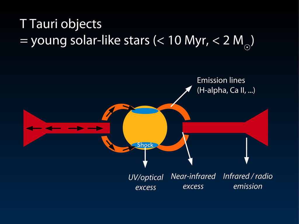
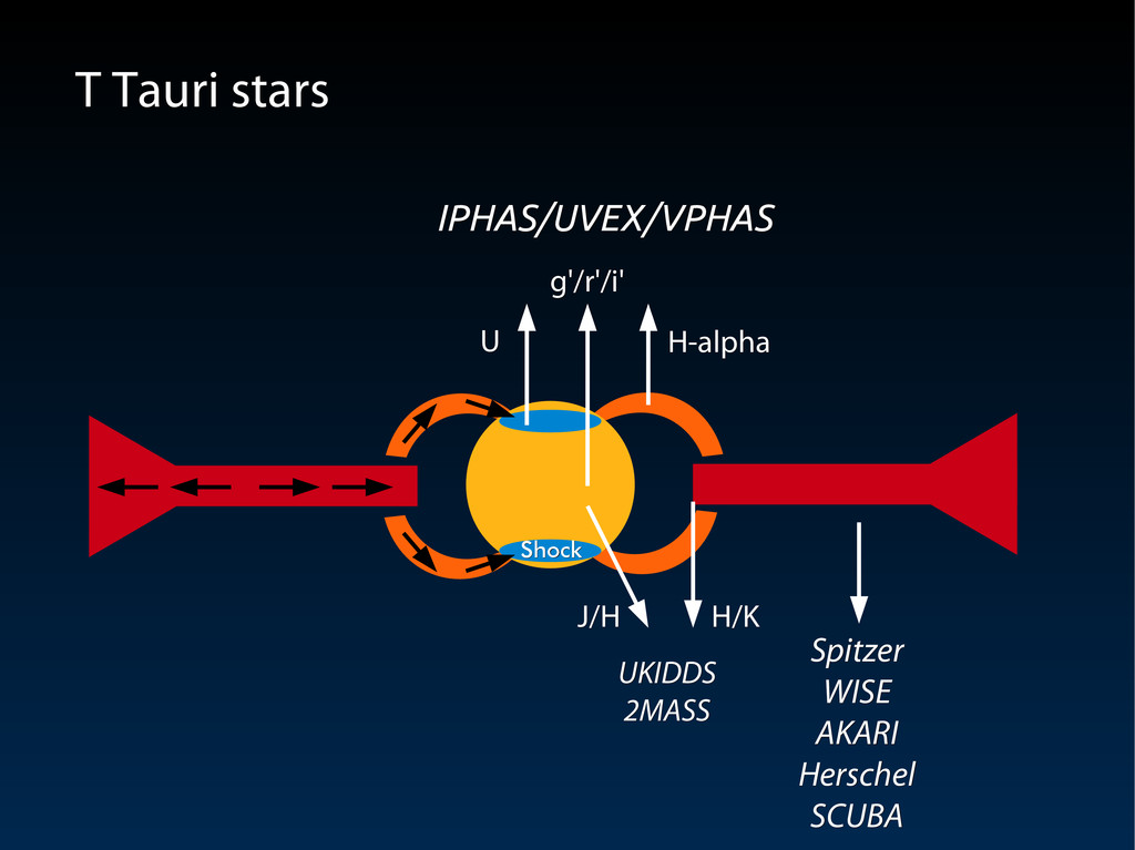
2. Shock Shock Infrared / radio Infrared / radio emission emission Near-infrared Near-infrared excess excess UV/optical UV/optical excess excess T Tauri objects T Tauri objects = young solar-like stars (< 10 Myr, = young solar-like stars (< 10 Myr, < 2 M < 2 M ☉ ☉ ) ) Emission lines Emission lines (H-alpha, Ca II, ...) (H-alpha, Ca II, ...)
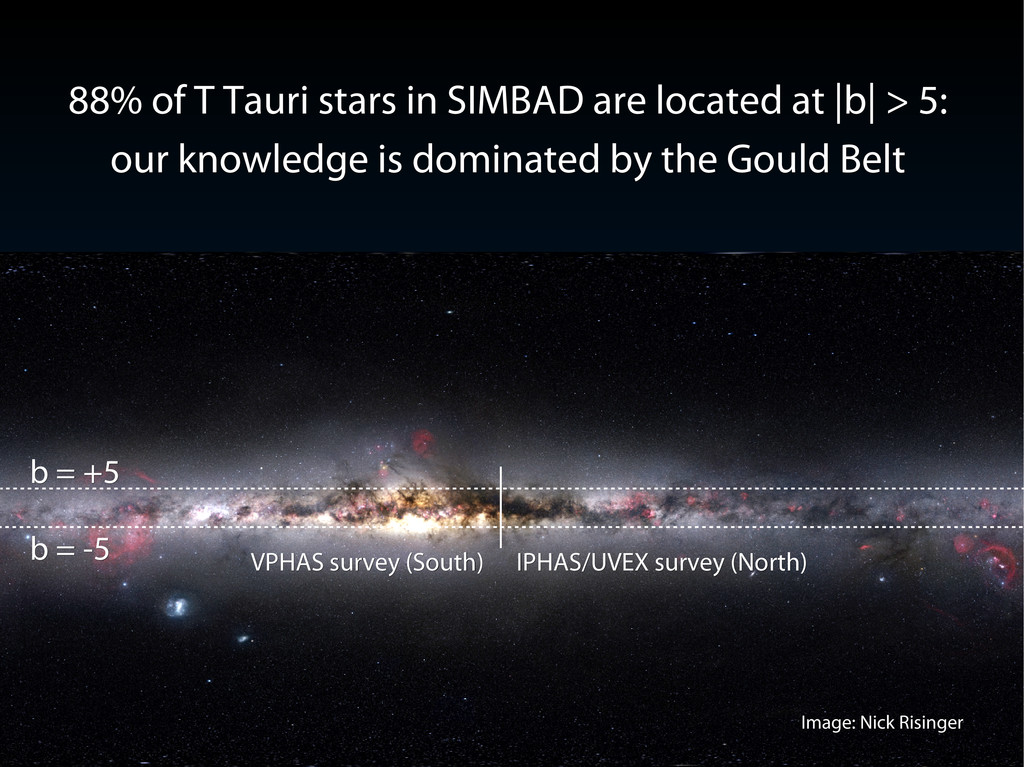
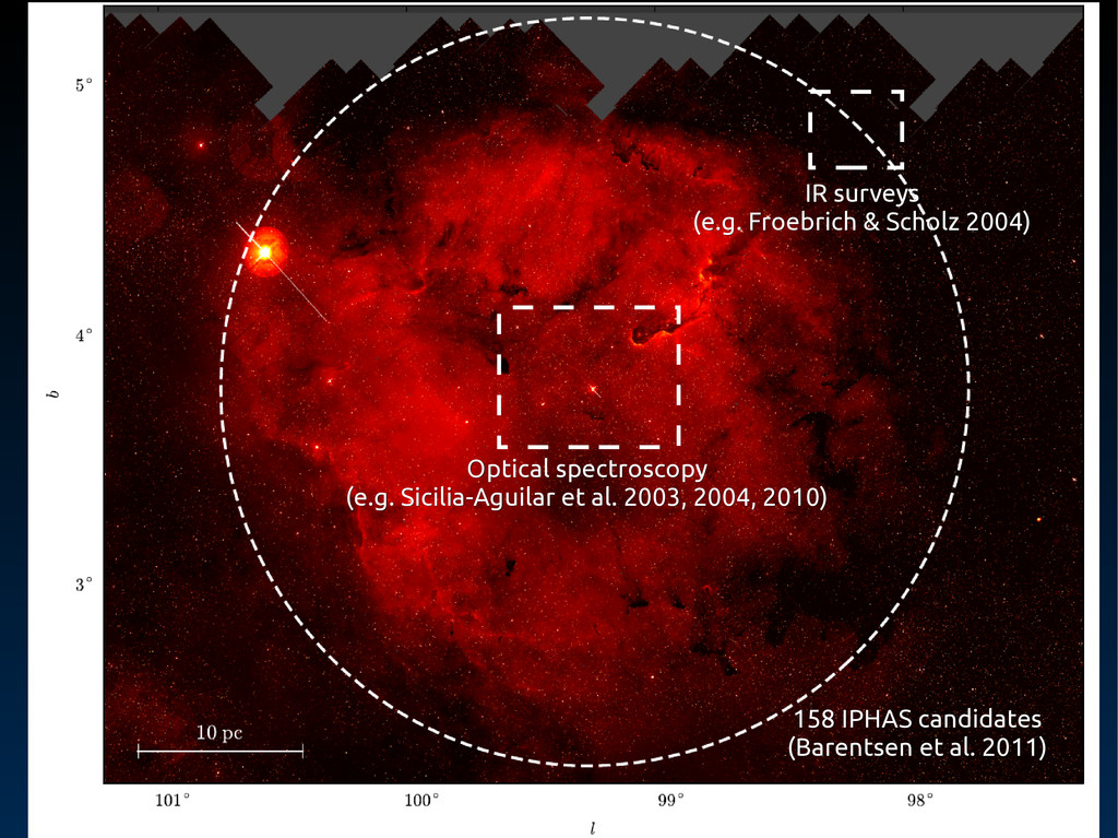
3. Image: Nick Risinger Image: Nick Risinger VPHAS survey (South) IPHAS/UVEX survey (North) VPHAS survey (South) IPHAS/UVEX survey (North) 88% of T Tauri stars in SIMBAD are located at |b| > 5: 88% of T Tauri stars in SIMBAD are located at |b| > 5: our knowledge is dominated by the Gould Belt our knowledge is dominated by the Gould Belt b = +5 b = +5 b = -5 b = -5
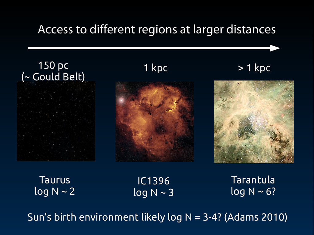
4. Taurus Taurus log N ~ 2 log N ~ 2 IC1396 IC1396 log N ~ 3 log N ~ 3 Tarantula Tarantula log N ~ 6? log N ~ 6? 150 pc 150 pc (~ Gould Belt) (~ Gould Belt) 1 kpc 1 kpc > 1 kpc > 1 kpc Access to different regions at larger distances Access to different regions at larger distances Sun's birth environment likely log N = 3-4? (Adams 2010) Sun's birth environment likely log N = 3-4? (Adams 2010)
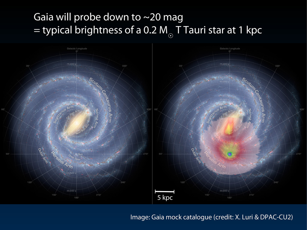
5. Gaia will probe down to ~20 mag Gaia will probe down to ~20 mag = typical brightness of a 0.2 M = typical brightness of a 0.2 M ☉ ☉ T Tauri star at 1 kpc T Tauri star at 1 kpc Image: Gaia mock catalogue (credit: X. Luri & DPAC-CU2) Image: Gaia mock catalogue (credit: X. Luri & DPAC-CU2) 5 kpc 5 kpc
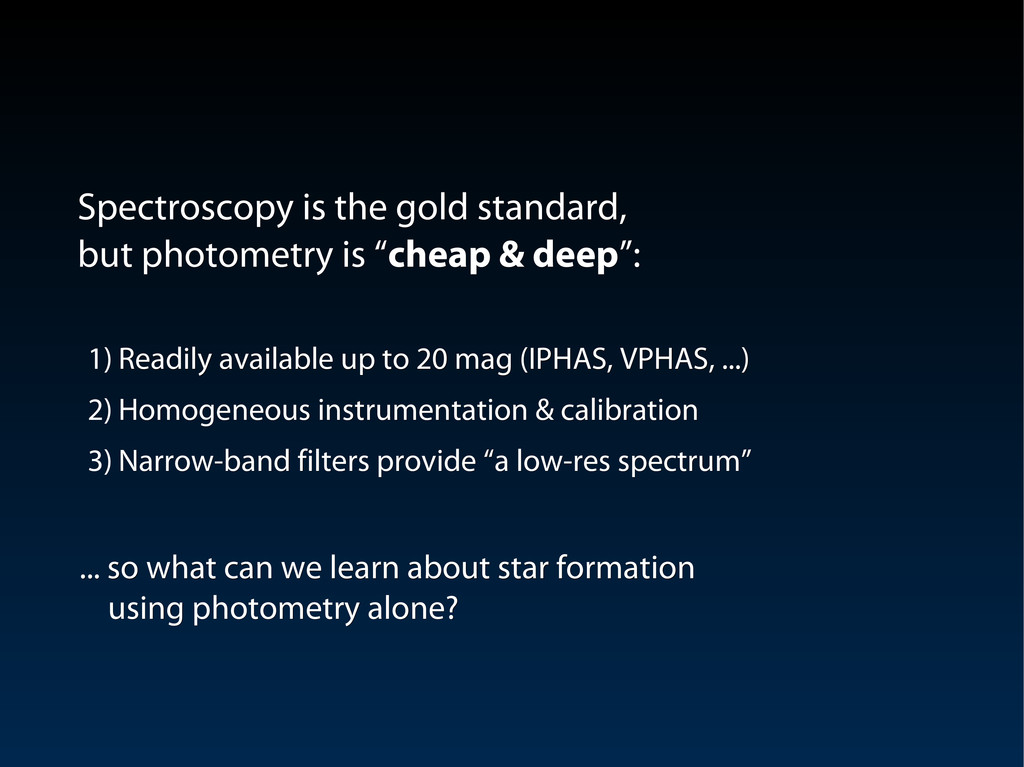
6. Spectroscopy is the gold standard, Spectroscopy is the gold standard, but photometry is “ but photometry is “cheap & deep cheap & deep”: ”: 1) Readily available up to 20 mag (IPHAS, VPHAS, ...) Readily available up to 20 mag (IPHAS, VPHAS, ...) 2) Homogeneous instrumentation & calibration Homogeneous instrumentation & calibration 3) Narrow-band filters provide “a low-res spectrum” Narrow-band filters provide “a low-res spectrum” ... so what can we learn about star formation ... so what can we learn about star formation using photometry alone? using photometry alone?
7. Shock Shock IPHAS/UVEX/VPHAS IPHAS/UVEX/VPHAS H-alpha H-alpha Spitzer Spitzer WISE WISE AKARI AKARI Herschel Herschel SCUBA SCUBA UKIDDS UKIDDS 2MASS 2MASS T Tauri stars T Tauri stars U U g'/r'/i' g'/r'/i' J/H J/H H/K H/K
8. Accretion Accretion rate rate
9. r'-i' / r'-Ha colour-colour diagram ~ H-alpha excess r'-i' / r'-Ha colour-colour diagram ~ H-alpha excess
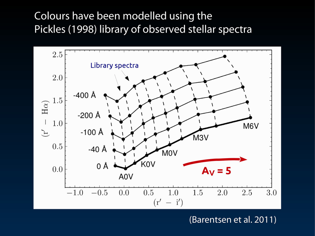
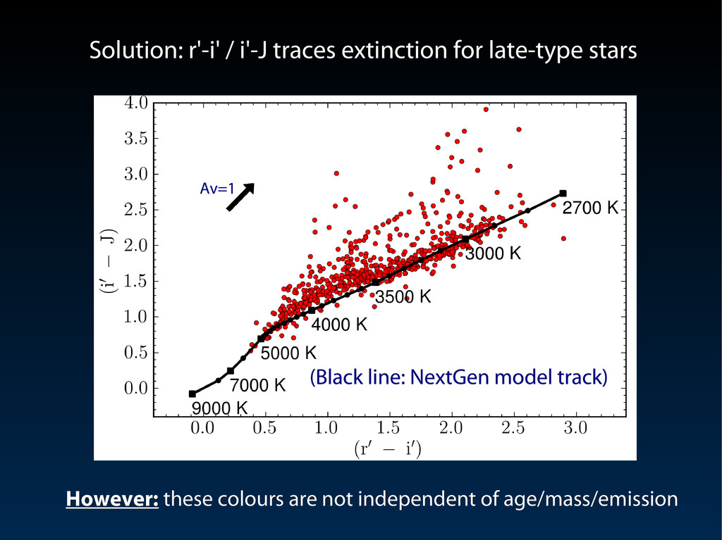
10. Library spectra Library spectra A AV V = 5 = 5 (Barentsen et al. 2011) (Barentsen et al. 2011) Colours have been modelled using the Colours have been modelled using the Pickles (1998) library of observed stellar spectra Pickles (1998) library of observed stellar spectra
11. H-alpha luminosity H-alpha luminosity Accretion Accretion luminosity luminosity H-alpha luminosity traces accretion luminosity H-alpha luminosity traces accretion luminosity (see De Marchi et al. 2010, 2011) (see De Marchi et al. 2010, 2011)
12. However: However: Emission-line stars suffer from Emission-line stars suffer from extinction degeneracy in the r'-i' / r-Ha plane extinction degeneracy in the r'-i' / r-Ha plane
13. r'-i' / r' colour-magnitude diagram ~ ages & masses r'-i' / r' colour-magnitude diagram ~ ages & masses isochrones isochrones However: However: colour-magnitude planes also suffer colour-magnitude planes also suffer from extinction degeneracy (common problem!) from extinction degeneracy (common problem!)
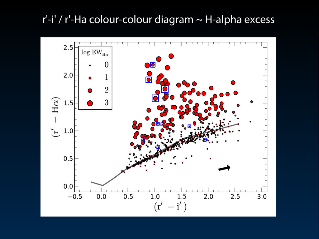
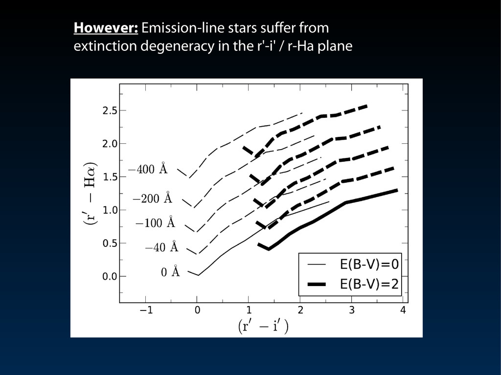
14. (Black line: NextGen model track) (Black line: NextGen model track) Solution: r'-i' / i'-J traces extinction for late-type stars Solution: r'-i' / i'-J traces extinction for late-type stars However: However: these colours are not independent of age/mass/emission these colours are not independent of age/mass/emission Av=1 Av=1
16. Problem statement Problem statement Given IPHAS/2MASS survey photometry Given IPHAS/2MASS survey photometry { r', Ha, i', J } { { r', Ha, i', J } { σ σ r' r' , , σ σ Ha Ha , , σ σ i' i' , , σ σ J J } } we aim to we aim to constrain constrain { Extinction, Mass, Age, Accretion rate } { Extinction, Mass, Age, Accretion rate } taking “nuisance parameters” into account taking “nuisance parameters” into account • Distance (760 Distance (760 ± ± 5 pc) 5 pc) • Inner disc radius (5 Inner disc radius (5 ± ± 2 R 2 R* * ) ) • log L log LHa Ha ~ log L ~ log Laccretion accretion ( (± ±0.43 dex) 0.43 dex)
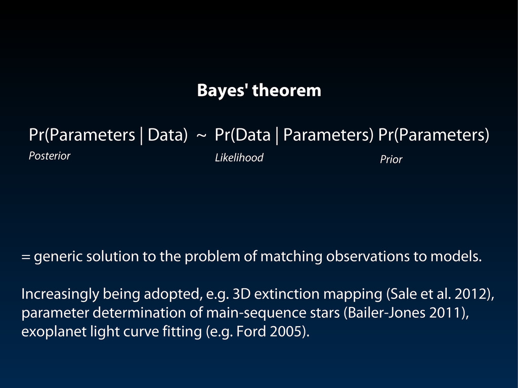
17. Bayes' theorem Bayes' theorem Pr(Parameters | Data) ~ Pr(Data | Parameters) Pr(Parameters) Pr(Parameters | Data) ~ Pr(Data | Parameters) Pr(Parameters) Likelihood Likelihood Prior Prior Posterior Posterior = generic solution to the problem of matching observations to models. = generic solution to the problem of matching observations to models. Increasingly being adopted, e.g. 3D extinction mapping (Sale et al. 2012), Increasingly being adopted, e.g. 3D extinction mapping (Sale et al. 2012), parameter determination of main-sequence stars (Bailer-Jones 2011), parameter determination of main-sequence stars (Bailer-Jones 2011), exoplanet light curve fitting (e.g. Ford 2005). exoplanet light curve fitting (e.g. Ford 2005).
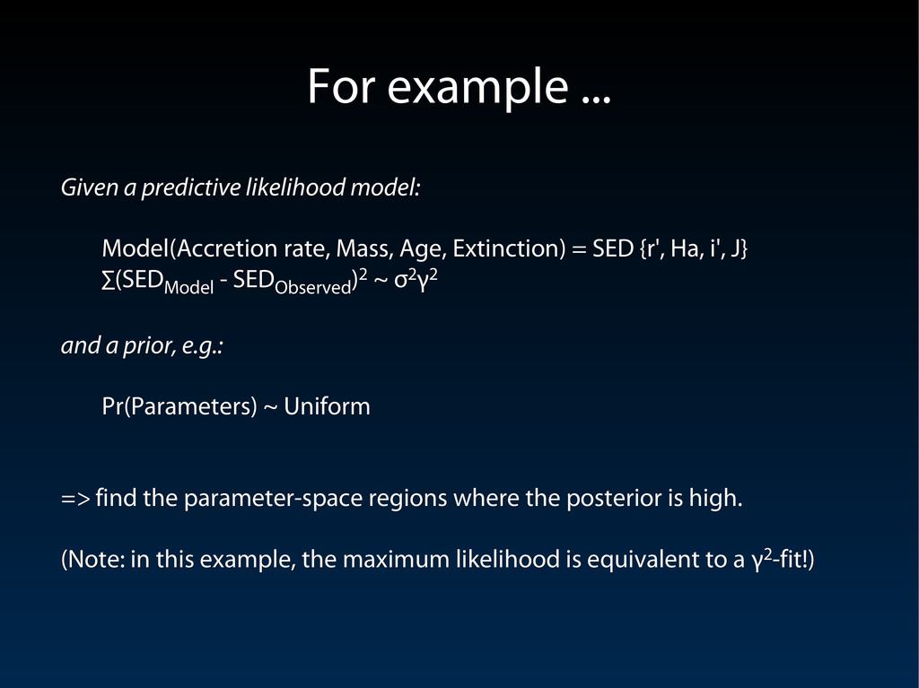
18. Given a predictive likelihood model: Given a predictive likelihood model: Model(Accretion rate, Mass, Age, Extinction) = SED {r', Ha, i', J} Model(Accretion rate, Mass, Age, Extinction) = SED {r', Ha, i', J} ∑ ∑(SED (SED Model Model - SED - SED Observed Observed ) )2 2 ~ ~ σ σ2 2γ γ2 2 and a prior, e.g.: and a prior, e.g.: Pr(Parameters) ~ Uniform Pr(Parameters) ~ Uniform => => find the parameter-space regions where the posterior is high. find the parameter-space regions where the posterior is high. (Note: in this example, the maximum likelihood is equivalent to a (Note: in this example, the maximum likelihood is equivalent to a γ γ2 2-fit!) -fit!) For example ... For example ...
19. = maximum likelihood method = maximum likelihood method = fast and hence very useful when data and model = fast and hence very useful when data and model uncertainties are small, uncertainties are small, but: but: 1) Photometric data is sparse Photometric data is sparse there is a family of degenerate solutions! there is a family of degenerate solutions! 2) Models are uncertain Models are uncertain the presence of “nuisance parameters” makes the the presence of “nuisance parameters” makes the likelihood more complicated than a Gaussian likelihood more complicated than a Gaussian => Estimate the full posterior distribution Pr(Parameters | Data) => Estimate the full posterior distribution Pr(Parameters | Data) So, why not simply use So, why not simply use γ γ2 2 fitting? fitting?
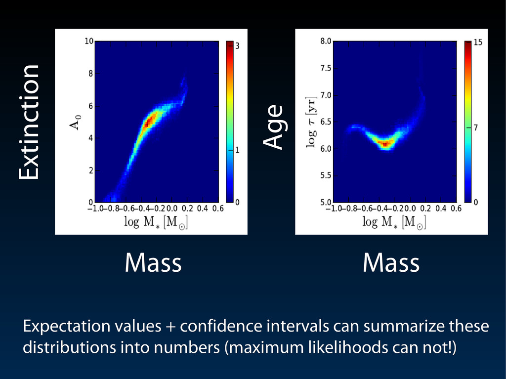
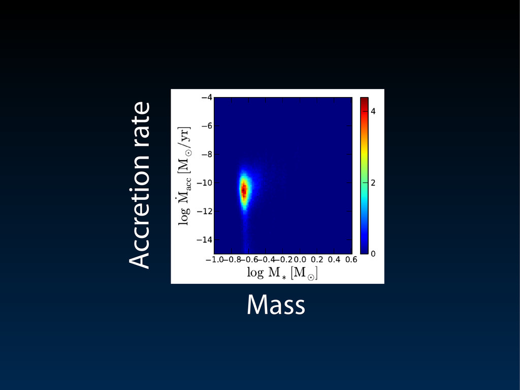
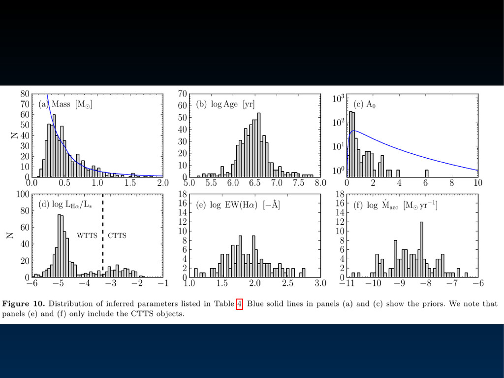
20. Expectation values + confidence intervals can summarize these Expectation values + confidence intervals can summarize these distributions into numbers (maximum likelihoods can not!) distributions into numbers (maximum likelihoods can not!) Mass Mass Mass Mass Extinction Extinction Age Age
21. Mass Mass Accretion rate Accretion rate
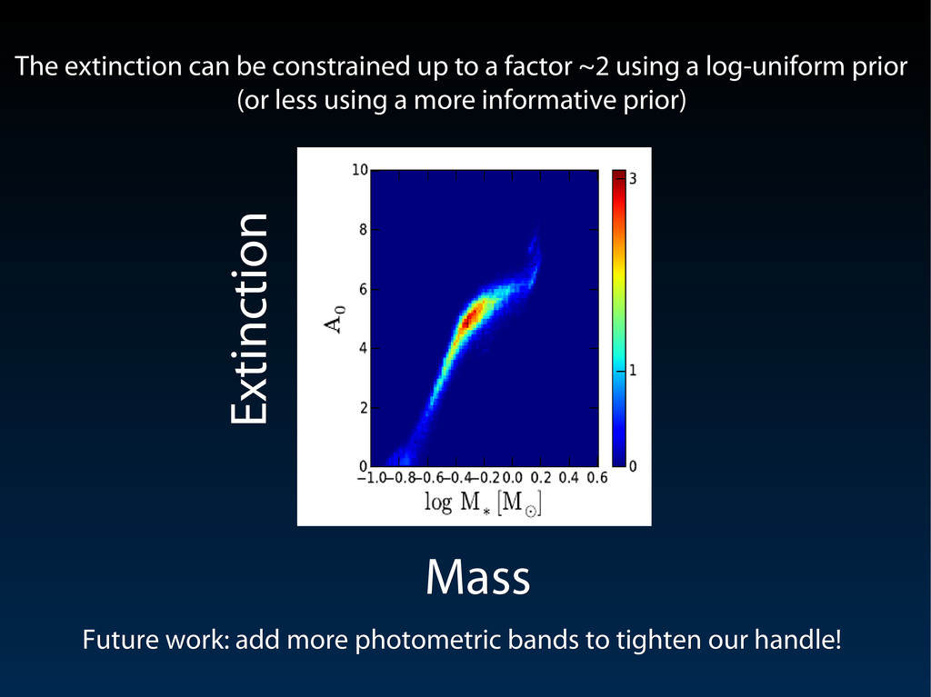
22. The extinction can be constrained up to a factor ~2 using a log-uniform prior The extinction can be constrained up to a factor ~2 using a log-uniform prior (or less using a more informative prior) (or less using a more informative prior) Mass Mass Extinction Extinction Future work: add more photometric bands to tighten our handle! Future work: add more photometric bands to tighten our handle!
23. How to define a Bayesian (probabilistic) model? How to define a Bayesian (probabilistic) model?
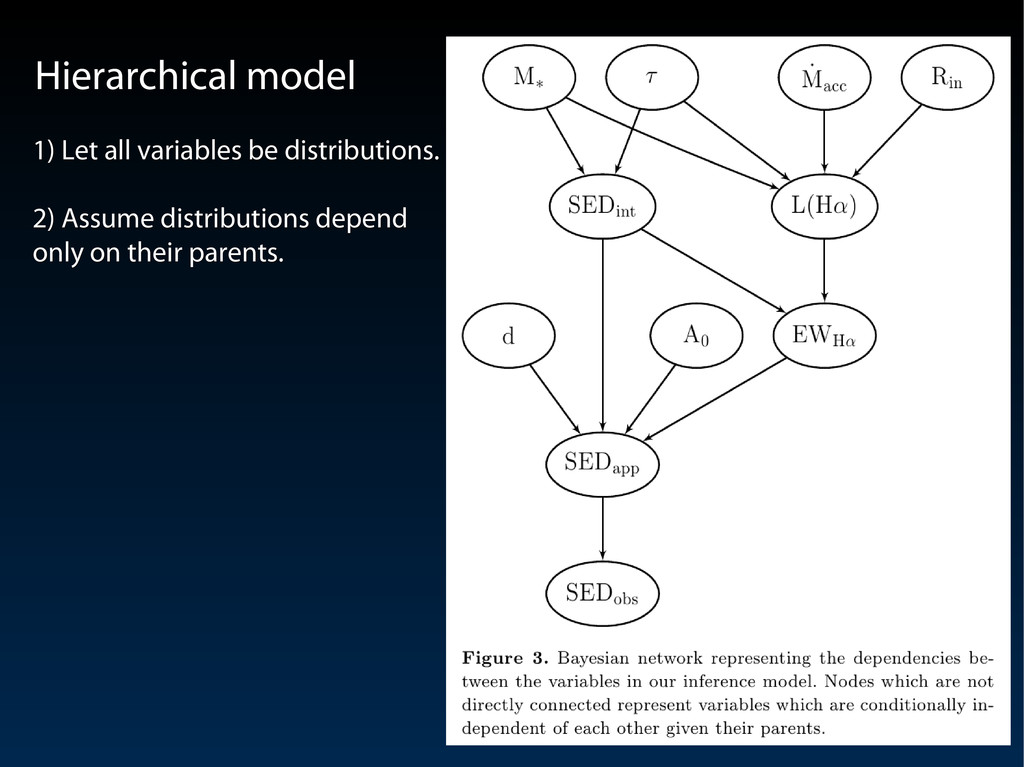
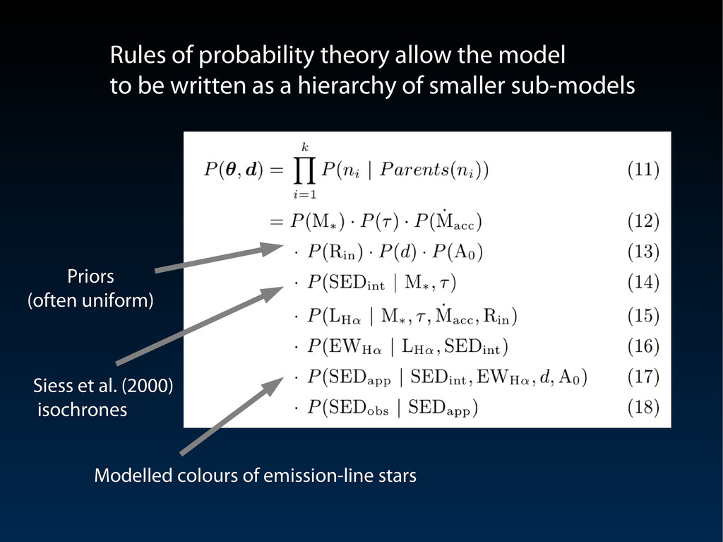
24. 1) Let all variables be distributions. 1) Let all variables be distributions. 2) Assume distributions depend 2) Assume distributions depend only on their parents. only on their parents. Hierarchical model Hierarchical model
25. Siess et al. (2000) Siess et al. (2000) isochrones isochrones Modelled colours of emission-line stars Modelled colours of emission-line stars Rules of probability theory allow the model Rules of probability theory allow the model to be written as a hierarchy of smaller sub-models to be written as a hierarchy of smaller sub-models Priors Priors (often uniform) (often uniform)
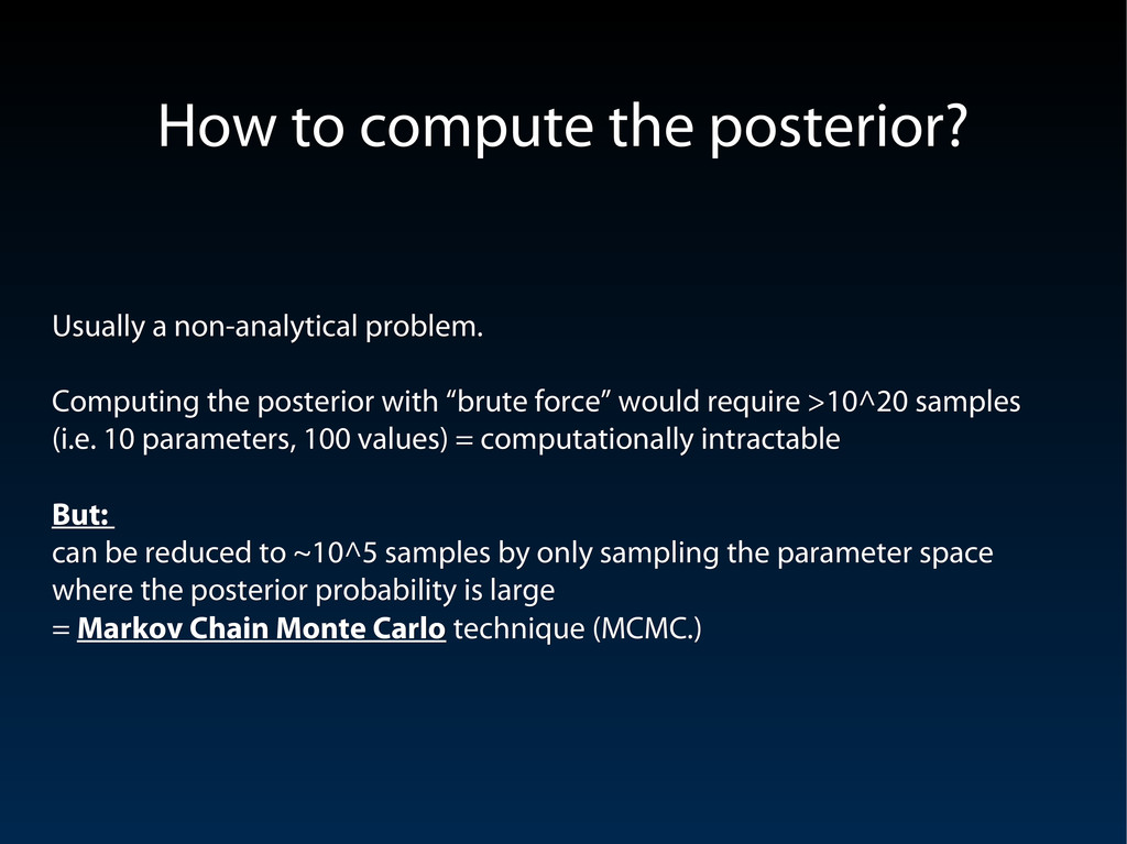
26. Usually a non-analytical problem. Usually a non-analytical problem. Computing the posterior with “brute force” would require >10^20 samples Computing the posterior with “brute force” would require >10^20 samples (i.e. 10 parameters, 100 values) = computationally intractable (i.e. 10 parameters, 100 values) = computationally intractable But: But: can be reduced to ~10^5 samples by only sampling the parameter space can be reduced to ~10^5 samples by only sampling the parameter space where the posterior probability is large where the posterior probability is large = = Markov Chain Monte Carlo Markov Chain Monte Carlo technique (MCMC.) technique (MCMC.) How to compute the posterior? How to compute the posterior?
27. http://github.com/barentsen/astro http://github.com/barentsen/astro Pythonic (i.e. minimal effort) implementation using Python/PyMC Pythonic (i.e. minimal effort) implementation using Python/PyMC
28. Application Application
29. 2 degrees = 30 pc (d ~ 900 pc) 2 degrees = 30 pc (d ~ 900 pc) O6V-type O6V-type IC1396 IPHAS mosaic IC1396 IPHAS mosaic
30. 30“ 30“ IPHAS H-alpha IPHAS H-alpha
31. Optical spectroscopy Optical spectroscopy (e.g. Sicilia-Aguilar et al. 2003, 2004, 2010) (e.g. Sicilia-Aguilar et al. 2003, 2004, 2010) 158 IPHAS candidates 158 IPHAS candidates (Barentsen et al. 2011) (Barentsen et al. 2011) IR surveys IR surveys (e.g. Froebrich & Scholz 2004) (e.g. Froebrich & Scholz 2004)
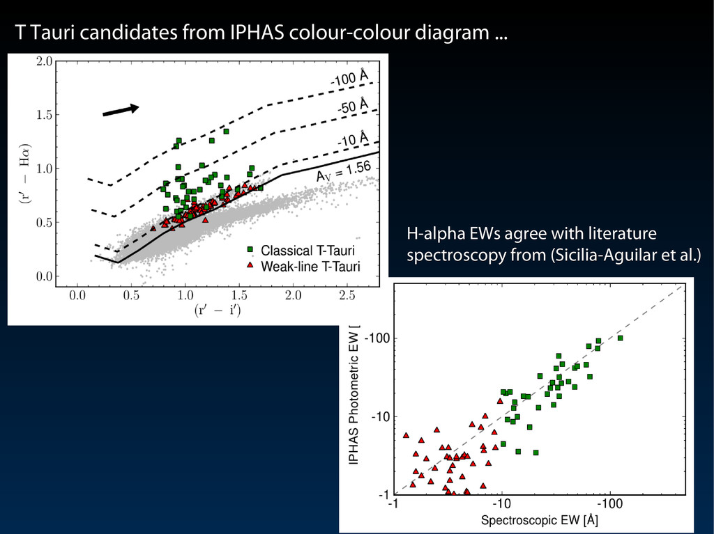
32. T Tauri candidates from IPHAS colour-colour diagram ... T Tauri candidates from IPHAS colour-colour diagram ... H-alpha EWs agree with literature H-alpha EWs agree with literature spectroscopy from (Sicilia-Aguilar et al.) spectroscopy from (Sicilia-Aguilar et al.)
33. Result: stellar parameters and accretion rates for 158 candidates Result: stellar parameters and accretion rates for 158 candidates
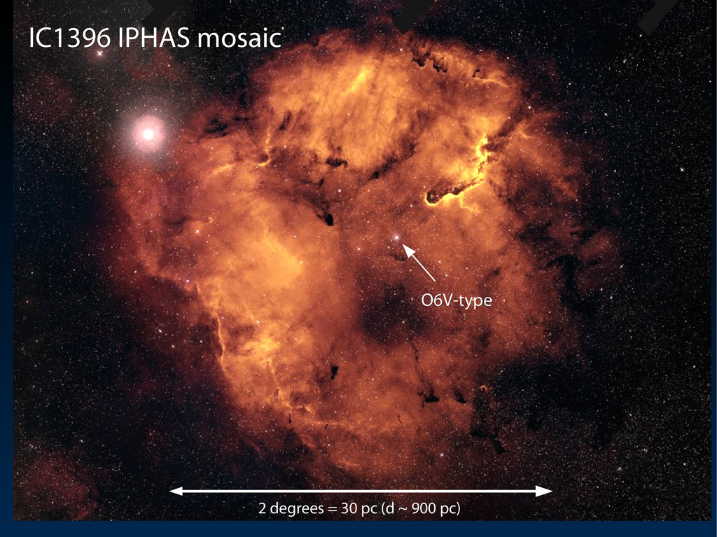
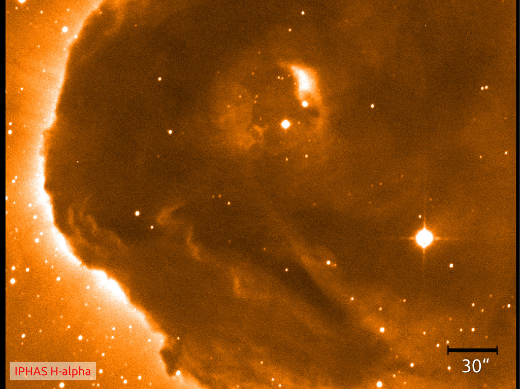
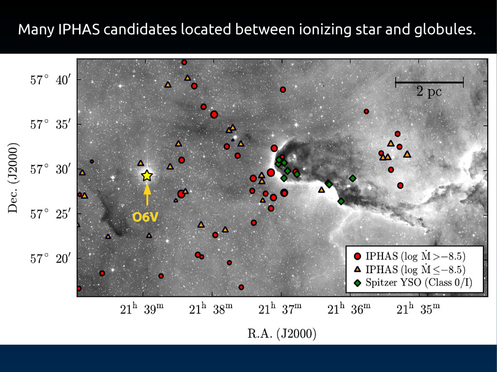
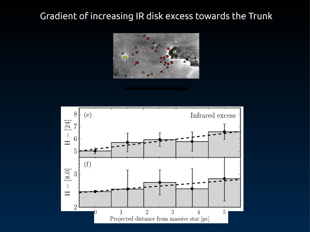
34. IPHAS objects IPHAS objects (2-3 Myr) (2-3 Myr) Spitzer YSOs Spitzer YSOs (< 1 Myr) (< 1 Myr) Hot star Hot star The spatial dispersion of objects in front of the globules suggests an The spatial dispersion of objects in front of the globules suggests an age gradient away from the central O-type star age gradient away from the central O-type star Consistent with Consistent with sequentially triggered star formation. sequentially triggered star formation. Detailed discussion in (Barentsen et al. 2011, MNRAS) Detailed discussion in (Barentsen et al. 2011, MNRAS)
35. IPHAS offers reliable data for 567 known members from (Sung et al. 2009). IPHAS offers reliable data for 567 known members from (Sung et al. 2009). NGC 2264 = Cone Nebula NGC 2264 = Cone Nebula
37. Preliminary conclusions on NGC 2264 Preliminary conclusions on NGC 2264 • Median age: 3.0 Myr Median age: 3.0 Myr • Accretor fraction: 20% (+/- 2%) Accretor fraction: 20% (+/- 2%) • Median accretion rate: 10 Median accretion rate: 10-8.4 -8.4 Msol / yr Msol / yr
38. IPHAS/VPHAS can provide alternative cluster age estimates IPHAS/VPHAS can provide alternative cluster age estimates
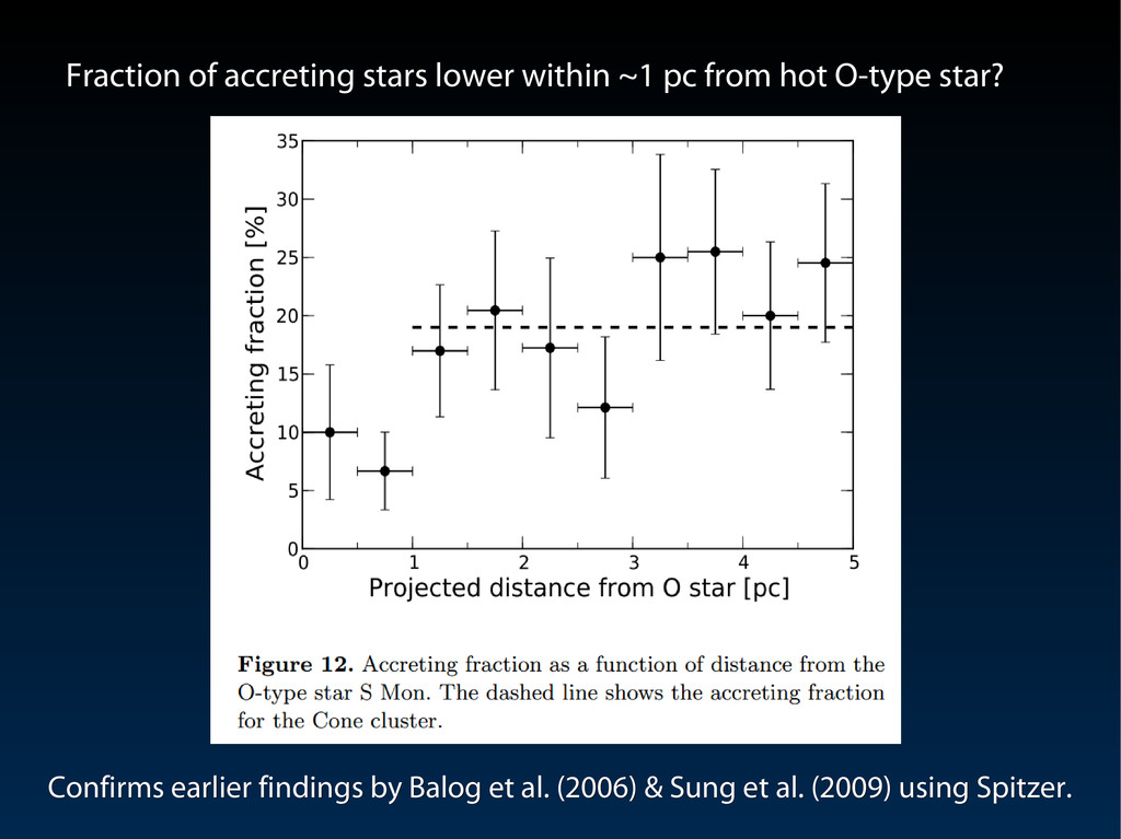
39. Confirms earlier findings by Balog et al. (2006) & Sung et al. (2009) using Spitzer. Confirms earlier findings by Balog et al. (2006) & Sung et al. (2009) using Spitzer. Fraction of accreting stars lower within ~1 pc from hot O-type star? Fraction of accreting stars lower within ~1 pc from hot O-type star?
40. Mass vs Accretion rate Mass vs Accretion rate
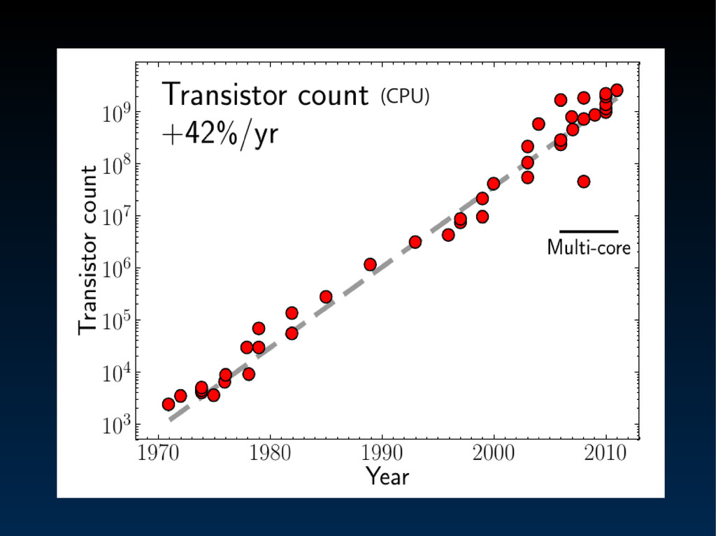
41. Conclusion Conclusion • Photometry is cheap & deep. Photometry is cheap & deep. • Large databases are waiting to be exploited. Large databases are waiting to be exploited. • Sophistication of knowledge inference tools is Sophistication of knowledge inference tools is increasingly becoming the limiting factor, rather increasingly becoming the limiting factor, rather than telescope time or processing power! than telescope time or processing power!
42. Future steps Future steps • Improve the likelihood model to include radiation transfer Improve the likelihood model to include radiation transfer models (circumstellar environment, accretion shock) models (circumstellar environment, accretion shock) • Incorporate additional surveys (UVEX, UKIDSS, Spitzer) Incorporate additional surveys (UVEX, UKIDSS, Spitzer) • Carry out a homogeneous, comparative study across Carry out a homogeneous, comparative study across Galactic star-forming regions Galactic star-forming regions (but need Gaia for accurate cluster membership lists) (but need Gaia for accurate cluster membership lists)
43. Backup slides Backup slides
44. Scientific progress is increasingly being limited Scientific progress is increasingly being limited by the sophistication of knowledge inference methods. by the sophistication of knowledge inference methods. Rather than by the amount of data or processing power. Rather than by the amount of data or processing power.
45. %/yr
46. (CPU)
47. O6V O6V Many IPHAS candidates located between ionizing star and globules. Many IPHAS candidates located between ionizing star and globules.
48. Gradient of increasing IR disk excess towards the Trunk Gradient of increasing IR disk excess towards the Trunk
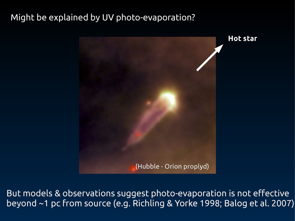
49. (Hubble - Orion proplyd) (Hubble - Orion proplyd) Might be explained by UV photo-evaporation? Might be explained by UV photo-evaporation? But models & observations suggest photo-evaporation is not effective But models & observations suggest photo-evaporation is not effective beyond ~1 pc from source (e.g. Richling & Yorke 1998; Balog et al. 2007) beyond ~1 pc from source (e.g. Richling & Yorke 1998; Balog et al. 2007) Hot star Hot star
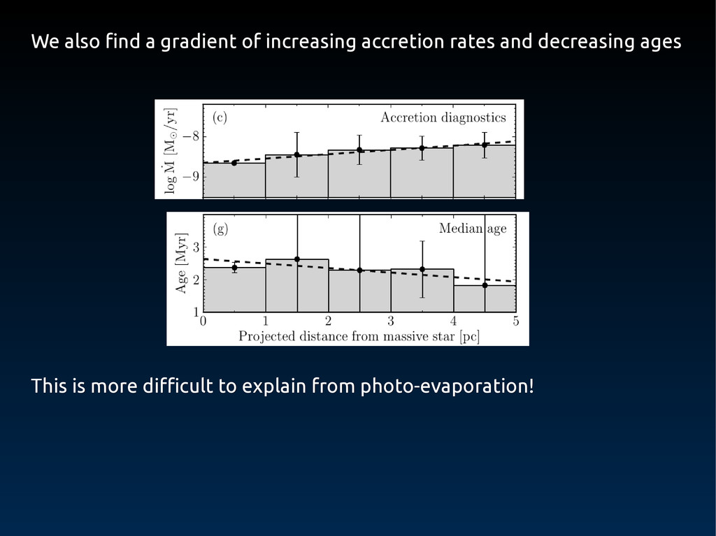
50. We also find a gradient of increasing accretion rates and decreasing ages We also find a gradient of increasing accretion rates and decreasing ages This is more difficult to explain from photo-evaporation! This is more difficult to explain from photo-evaporation!