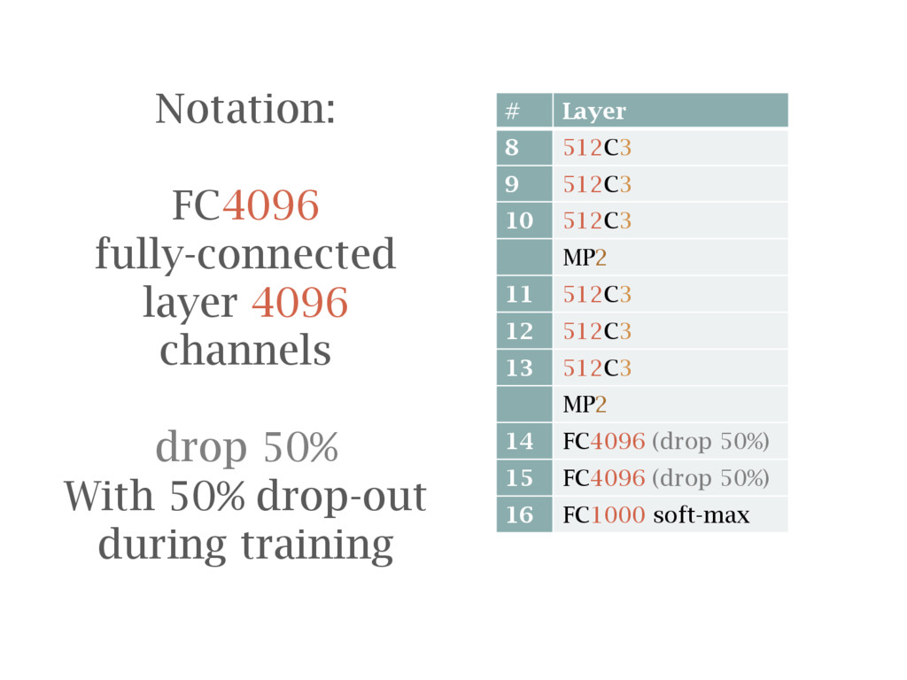
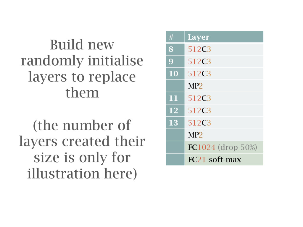
convolutional network trained by the VGG group at Oxford University Transfer learning Re-using pre-trained networks Deep learning tricks of the trade tips to save you some time
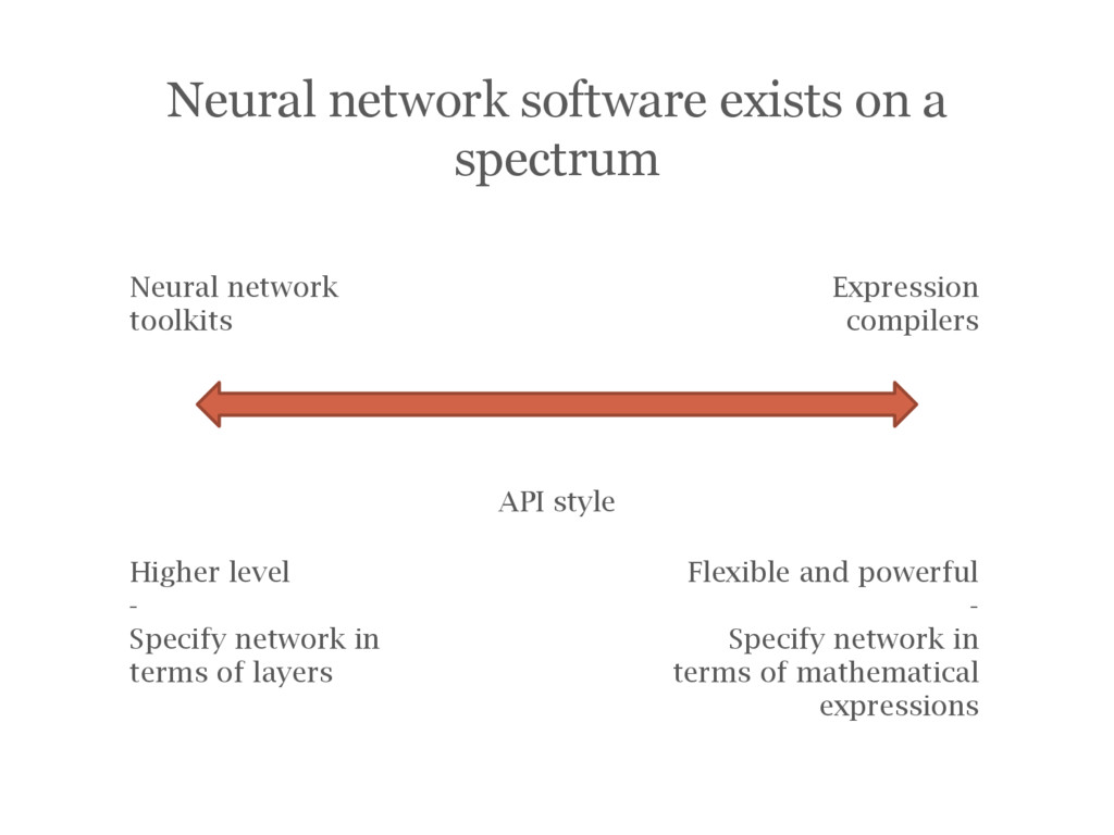
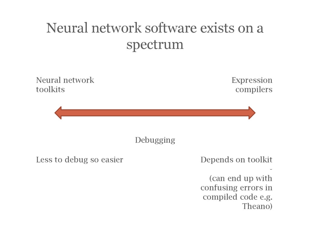
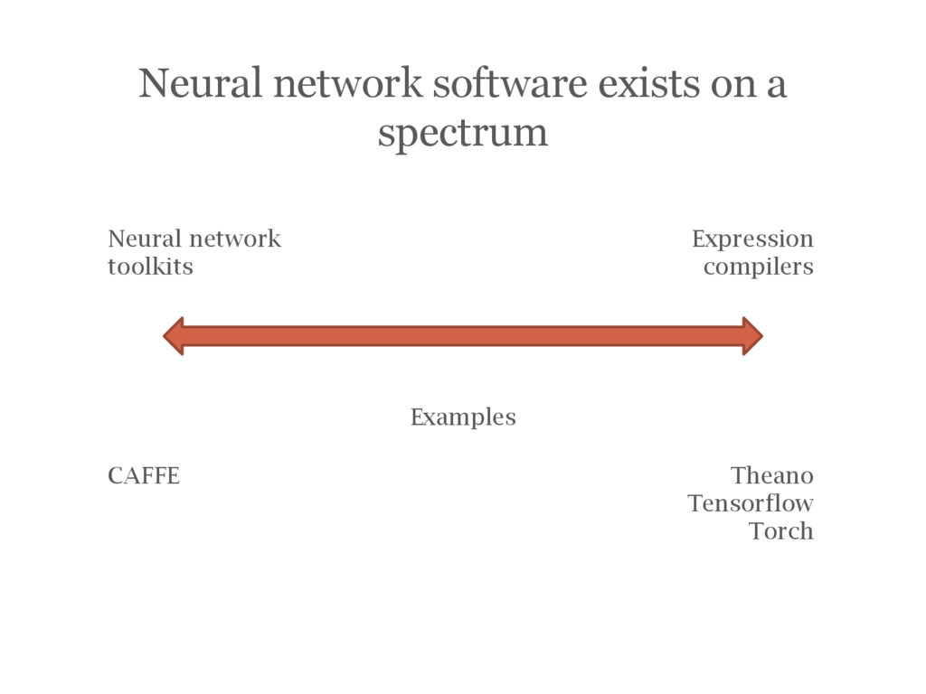
Specify network in terms of layers Flexible and powerful - Specify network in terms of mathematical expressions Neural network toolkits Expression compilers API style
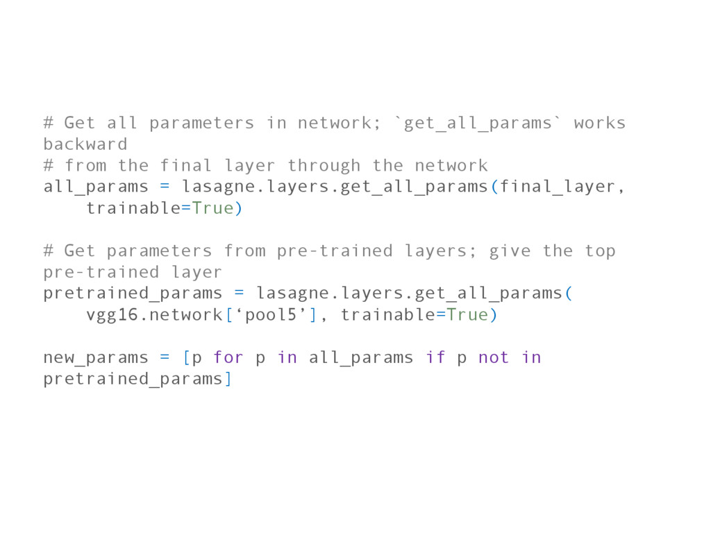
from the final layer through the network all_params = lasagne.layers.get_all_params(final_layer, trainable=True) # Get parameters from pre-trained layers; give the top pre-trained layer pretrained_params = lasagne.layers.get_all_params( vgg16.network[‘pool5’], trainable=True) new_params = [p for p in all_params if p not in pretrained_params]
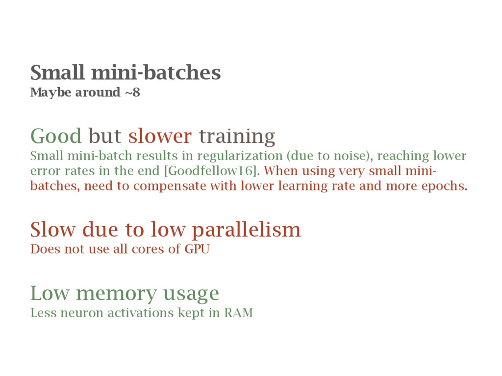
mini-batch results in regularization (due to noise), reaching lower error rates in the end [Goodfellow16]. When using very small mini- batches, need to compensate with lower learning rate and more epochs. Slow due to low parallelism Does not use all cores of GPU Low memory usage Less neuron activations kept in RAM
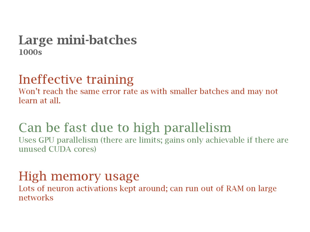
rate as with smaller batches and may not learn at all. Can be fast due to high parallelism Uses GPU parallelism (there are limits; gains only achievable if there are unused CUDA cores) High memory usage Lots of neuron activations kept around; can run out of RAM on large networks
lots of experiments use ~100 Effective training Learns reasonably quickly – in terms of improvement per epoch – and reaches acceptable error rate or loss Medium performance Acceptable in many cases Medium memory usage Fine for modest sized networks
15] Train two networks; one given random parameters to generate an image, another to discriminate between a generated image and one from the training set
model [Simonyan14] and extract texture features from one of the convolutional layers, given a target style / painting as input Use gradient descent to iterate photo – not weights – so that its texture features match those of the target image.
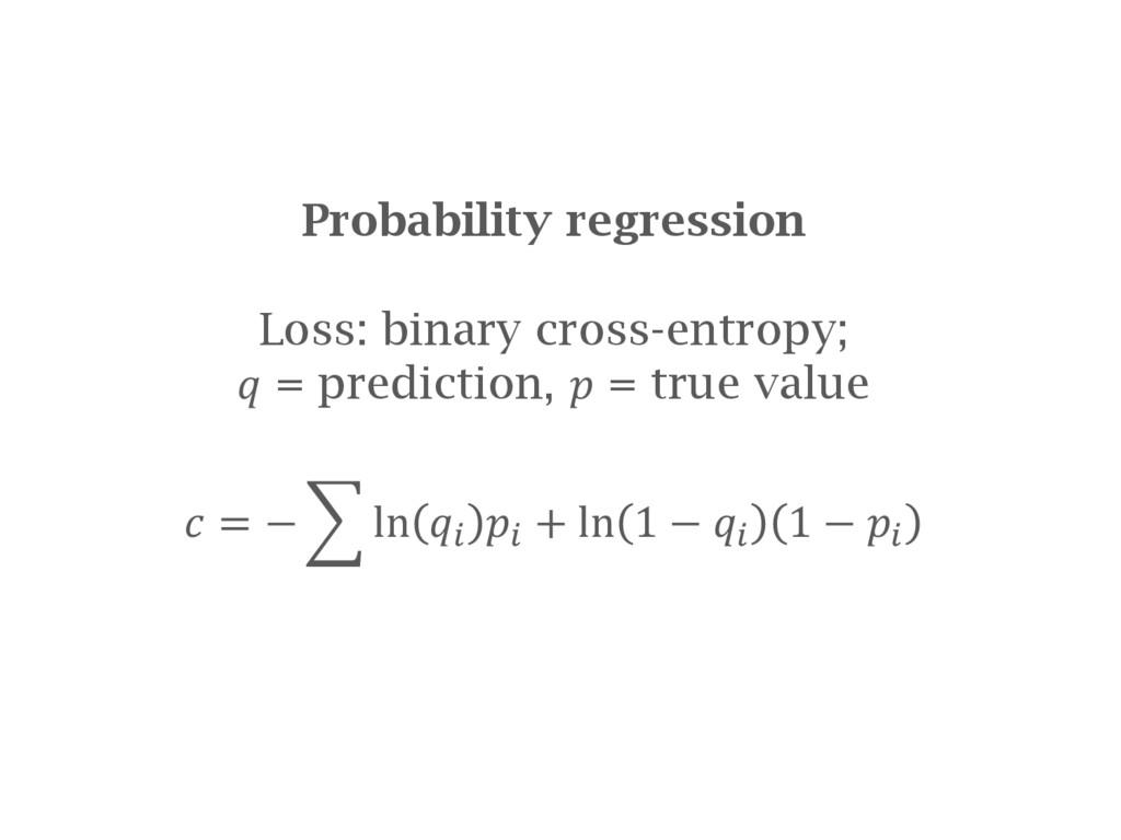
![Probability regression Use for predicting single value in [0, 1]](https://files.speakerdeck.com/presentations/8a0569b3e7644f4aa0520d3f98aafb9c/slide_44.jpg)
![Down-sampling: max-pooling ‘layer’ [Ciresan12] Take maximum value from each 2](https://files.speakerdeck.com/presentations/8a0569b3e7644f4aa0520d3f98aafb9c/slide_78.jpg)
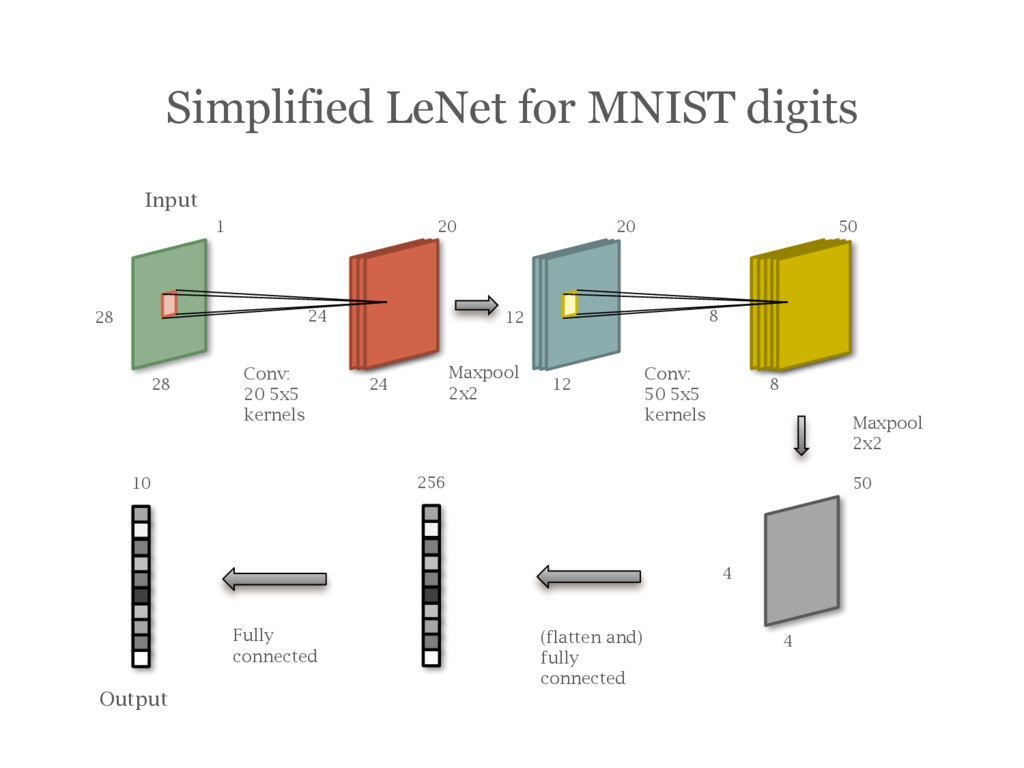
![Example: A Simplified LeNet [LeCun95] for MNIST digits](https://files.speakerdeck.com/presentations/8a0569b3e7644f4aa0520d3f98aafb9c/slide_80.jpg)
![Batch normalization [Ioffe15] is recommended in most cases Speeds up](https://files.speakerdeck.com/presentations/8a0569b3e7644f4aa0520d3f98aafb9c/slide_159.jpg)
![Can be partially addressed with careful weight initialization [He15]. Batch](https://files.speakerdeck.com/presentations/8a0569b3e7644f4aa0520d3f98aafb9c/slide_165.jpg)
![See [Krizhevsky12]; their paper discusses their techniques, that have since](https://files.speakerdeck.com/presentations/8a0569b3e7644f4aa0520d3f98aafb9c/slide_192.jpg)
![Visualizing and understanding convolutional networks [Zeiler14] Visualisations of responses of](https://files.speakerdeck.com/presentations/8a0569b3e7644f4aa0520d3f98aafb9c/slide_228.jpg)
![Visualizing and understanding convolutional networks [Zeiler14] Image taken from [Zeiler14]](https://files.speakerdeck.com/presentations/8a0569b3e7644f4aa0520d3f98aafb9c/slide_229.jpg)
![Visualizing and understanding convolutional networks [Zeiler14] Image taken from [Zeiler14]](https://files.speakerdeck.com/presentations/8a0569b3e7644f4aa0520d3f98aafb9c/slide_230.jpg)
![Learning to generate chairs with convolutional neural networks [Dosovitskiy15] Network](https://files.speakerdeck.com/presentations/8a0569b3e7644f4aa0520d3f98aafb9c/slide_234.jpg)
![Learning to generate chairs with convolutional neural networks [Dosovitskiy15] Image](https://files.speakerdeck.com/presentations/8a0569b3e7644f4aa0520d3f98aafb9c/slide_235.jpg)
![Generative Adversarial Nets [Radford15] Images of bedrooms generated using neural](https://files.speakerdeck.com/presentations/8a0569b3e7644f4aa0520d3f98aafb9c/slide_237.jpg)
![Generative Adversarial Nets [Radford15] Image taken from [Radford15]](https://files.speakerdeck.com/presentations/8a0569b3e7644f4aa0520d3f98aafb9c/slide_238.jpg)
![BEGAN:BoundaryEquilibriumGenerative AdversarialNetworks [Berthelot17] Image taken from [Berthelot17]](https://files.speakerdeck.com/presentations/8a0569b3e7644f4aa0520d3f98aafb9c/slide_240.jpg)
![A Neural Algorithm of Artistic Style [Gatys15] Take an OxfordNet](https://files.speakerdeck.com/presentations/8a0569b3e7644f4aa0520d3f98aafb9c/slide_241.jpg)
![A Neural Algorithm of Artistic Style [Gatys15] Image taken from](https://files.speakerdeck.com/presentations/8a0569b3e7644f4aa0520d3f98aafb9c/slide_242.jpg)
![Deep Photo Style Transfer [Luan17] (also iterative, but just awesome)](https://files.speakerdeck.com/presentations/8a0569b3e7644f4aa0520d3f98aafb9c/slide_244.jpg)
![[Berthelot17] Berthelot D., Schumm T., Metz L.; “BEGAN: Boundary Equilibrium](https://files.speakerdeck.com/presentations/8a0569b3e7644f4aa0520d3f98aafb9c/slide_248.jpg)
![[Girshick15] Girshick, Ross; “Fast R- CNN”, Proceedings of the IEEE](https://files.speakerdeck.com/presentations/8a0569b3e7644f4aa0520d3f98aafb9c/slide_249.jpg)
![[He15a] He, Zhang, Ren and Sun; “Delving Deep into Rectifiers:](https://files.speakerdeck.com/presentations/8a0569b3e7644f4aa0520d3f98aafb9c/slide_250.jpg)
![[He15b] He, Kaiming, et al. "Deep Residual Learning for Image](https://files.speakerdeck.com/presentations/8a0569b3e7644f4aa0520d3f98aafb9c/slide_251.jpg)
![[Hinton12] G.E. Hinton, N. Srivastava, A. Krizhevsky, I. Sutskever and](https://files.speakerdeck.com/presentations/8a0569b3e7644f4aa0520d3f98aafb9c/slide_252.jpg)
![[Ioffe15] Ioffe, S.; Szegedy C.. (2015). “Batch Normalization: Accelerating Deep](https://files.speakerdeck.com/presentations/8a0569b3e7644f4aa0520d3f98aafb9c/slide_253.jpg)
![[Jones87] Jones, J.P.; Palmer, L.A. (1987). "An evaluation of the](https://files.speakerdeck.com/presentations/8a0569b3e7644f4aa0520d3f98aafb9c/slide_254.jpg)
![[Lin13] Lin, Min, Qiang Chen, and Shuicheng Yan. "Network in](https://files.speakerdeck.com/presentations/8a0569b3e7644f4aa0520d3f98aafb9c/slide_255.jpg)
![[Luan17] Luan F., Paris S., Shechtman E., Bala K. “Deep](https://files.speakerdeck.com/presentations/8a0569b3e7644f4aa0520d3f98aafb9c/slide_256.jpg)
![[Krizhevsky12] Krizhevsky, A., Sutskever, I. and Hinton, G. E. "ImageNet](https://files.speakerdeck.com/presentations/8a0569b3e7644f4aa0520d3f98aafb9c/slide_257.jpg)
![[Nesterov83] Nesterov, Y. A method of solving a convex programming](https://files.speakerdeck.com/presentations/8a0569b3e7644f4aa0520d3f98aafb9c/slide_258.jpg)
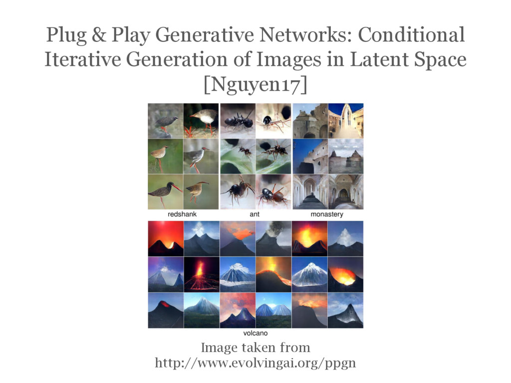
![[Nguyen17] Nguyen A., Yosinski J., Bengio Y., Dosovitskiy A., Clune](https://files.speakerdeck.com/presentations/8a0569b3e7644f4aa0520d3f98aafb9c/slide_259.jpg)
![[Sutskever13] Sutskever, Ilya, et al. On the importance of initialization](https://files.speakerdeck.com/presentations/8a0569b3e7644f4aa0520d3f98aafb9c/slide_260.jpg)
![[Simonyan14] K. Simonyan and Zisserman; “Very deep convolutional networks for](https://files.speakerdeck.com/presentations/8a0569b3e7644f4aa0520d3f98aafb9c/slide_261.jpg)
![[Wang14] Wang, Dan, and Yi Shang. "A new active labeling](https://files.speakerdeck.com/presentations/8a0569b3e7644f4aa0520d3f98aafb9c/slide_262.jpg)