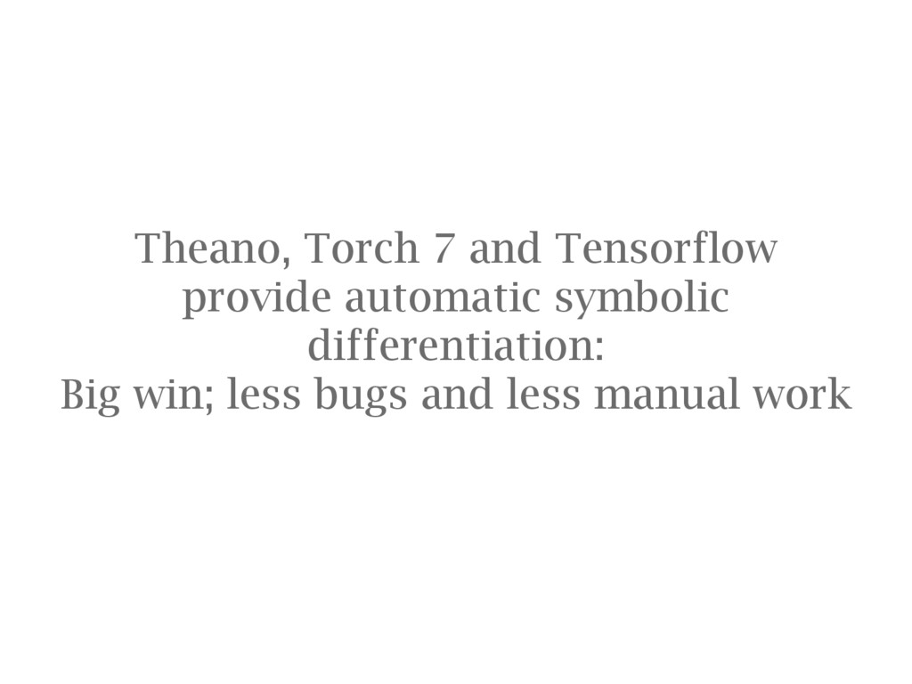
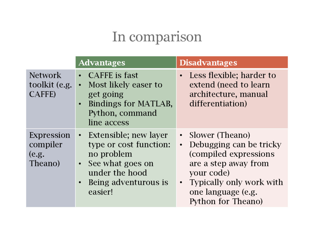
is fast • Most likely easer to get going • Bindings for MATLAB, Python, command line access • Less flexible; harder to extend (need to learn architecture, manual differentiation) Expression compiler (e.g. Theano) • Extensible; new layer type or cost function: no problem • See what goes on under the hood • Being adventurous is easier! • Slower (Theano) • Debugging can be tricky (compiled expressions are a step away from your code) • Typically only work with one language (e.g. Python for Theano)
model [Simonyan14] and extract texture features from one of the convolutional layers, given a target style / painting as input Use gradient descent to iterate photo – not weights – so that its texture features match those of the target image.
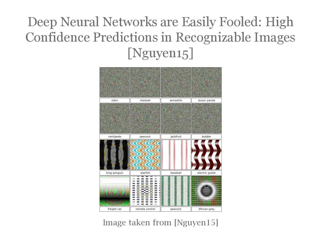
15] Train two networks; one given random parameters to generate an image, another to discriminate between a generated image and one from the training set
![Max-pooling ‘layer’ [Ciresan12] Take maximum value from each (, )](https://files.speakerdeck.com/presentations/50e4ae1058144e0daebfbdfd602d7e52/slide_56.jpg)
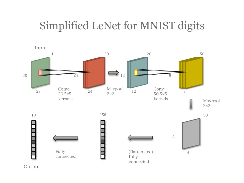
![A Simplified LeNet [LeCun95] for MNIST digits](https://files.speakerdeck.com/presentations/50e4ae1058144e0daebfbdfd602d7e52/slide_59.jpg)
![What about the learned kernels? Image taken from paper [Krizhevsky12]](https://files.speakerdeck.com/presentations/50e4ae1058144e0daebfbdfd602d7e52/slide_62.jpg)
![E.g. approach by He et. Al. [He15]: = 1 Where](https://files.speakerdeck.com/presentations/50e4ae1058144e0daebfbdfd602d7e52/slide_80.jpg)
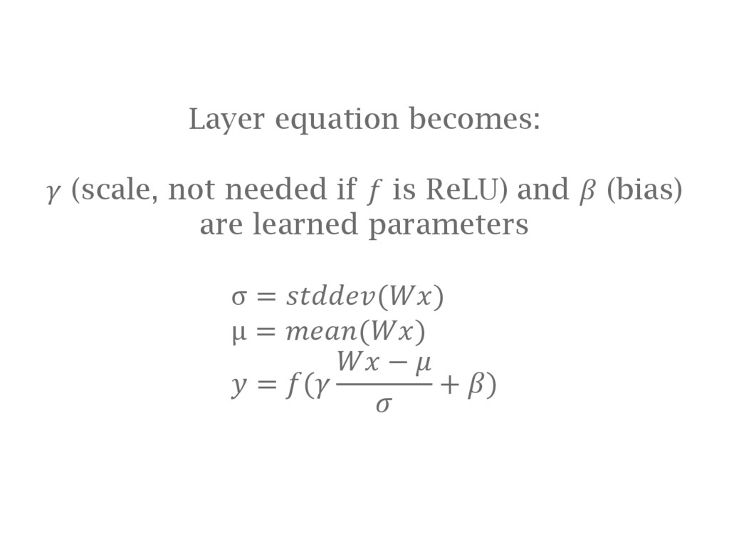
![New approach: BATCH NORMALISATION [Ioffe15] Keep distribution of activations sane](https://files.speakerdeck.com/presentations/50e4ae1058144e0daebfbdfd602d7e52/slide_81.jpg)
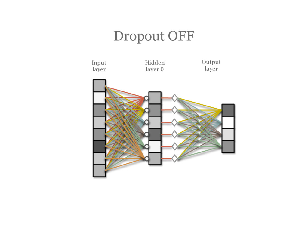
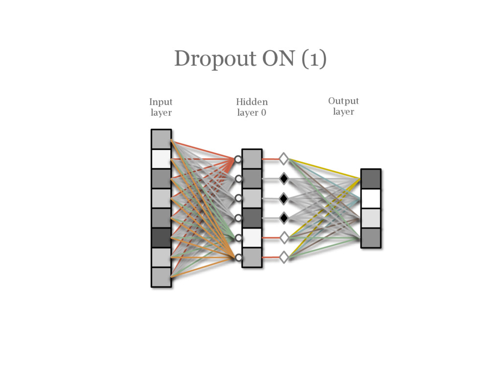
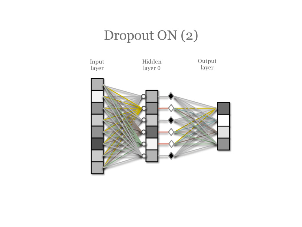
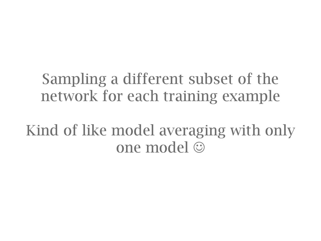
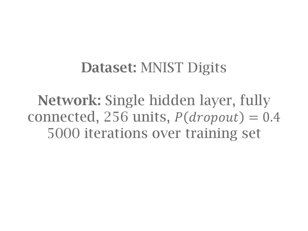
![DropOut [Hinton12] During training, randomly choose units to ‘drop out’](https://files.speakerdeck.com/presentations/50e4ae1058144e0daebfbdfd602d7e52/slide_91.jpg)
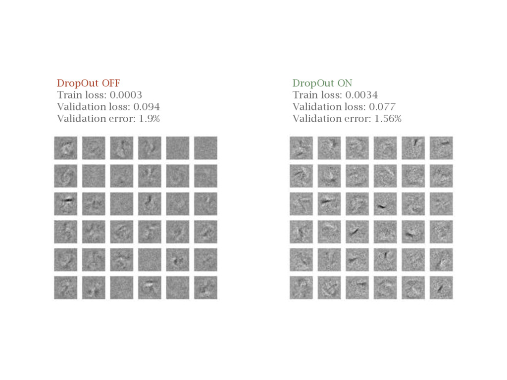
![What effect does it have? (approx. replication of [Hinton12])](https://files.speakerdeck.com/presentations/50e4ae1058144e0daebfbdfd602d7e52/slide_98.jpg)
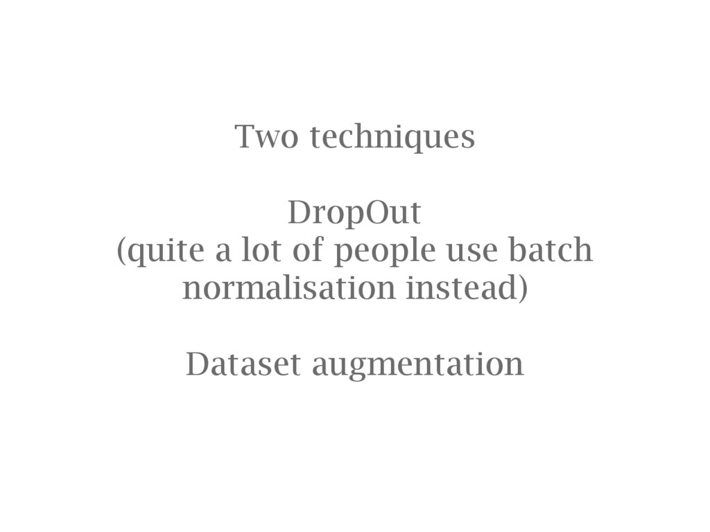
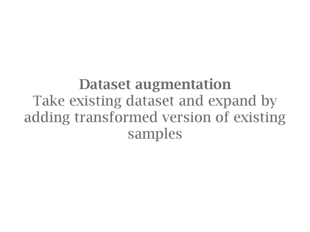
![Dataset augmentation for images [Krizhevsky12] Cropping and translation Scaling Rotation](https://files.speakerdeck.com/presentations/50e4ae1058144e0daebfbdfd602d7e52/slide_102.jpg)
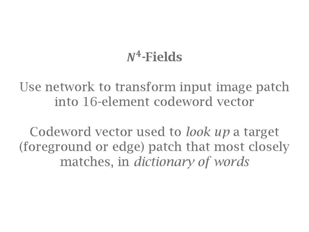
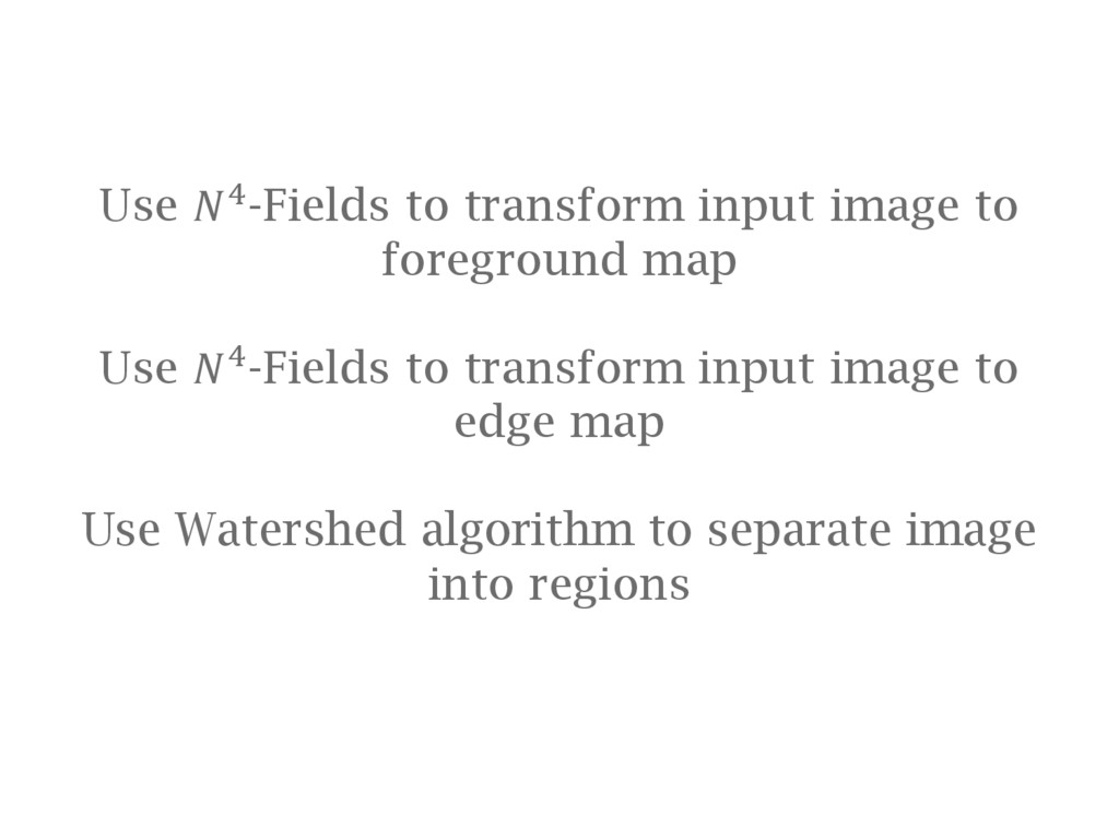
![Approach Use 4-Fields approach [Ganin14]](https://files.speakerdeck.com/presentations/50e4ae1058144e0daebfbdfd602d7e52/slide_123.jpg)
![Visualizing and understanding convolutional networks [Zeiler14] Visualisations of responses of](https://files.speakerdeck.com/presentations/50e4ae1058144e0daebfbdfd602d7e52/slide_132.jpg)
![Visualizing and understanding convolutional networks [Zeiler14] Image taken from [Zeiler14]](https://files.speakerdeck.com/presentations/50e4ae1058144e0daebfbdfd602d7e52/slide_133.jpg)
![Visualizing and understanding convolutional networks [Zeiler14] Image taken from [Zeiler14]](https://files.speakerdeck.com/presentations/50e4ae1058144e0daebfbdfd602d7e52/slide_134.jpg)
![Learning to generate chairs with convolutional neural networks [Dosovitskiy15] Network](https://files.speakerdeck.com/presentations/50e4ae1058144e0daebfbdfd602d7e52/slide_137.jpg)
![Learning to generate chairs with convolutional neural networks [Dosovitskiy15] Image](https://files.speakerdeck.com/presentations/50e4ae1058144e0daebfbdfd602d7e52/slide_138.jpg)
![A Neural Algorithm of Artistic Style [Gatys15] Take an OxfordNet](https://files.speakerdeck.com/presentations/50e4ae1058144e0daebfbdfd602d7e52/slide_139.jpg)
![A Neural Algorithm of Artistic Style [Gatys15] Image taken from](https://files.speakerdeck.com/presentations/50e4ae1058144e0daebfbdfd602d7e52/slide_140.jpg)
![Generative Adversarial Nets [Radford15] Images of bedrooms generated using neural](https://files.speakerdeck.com/presentations/50e4ae1058144e0daebfbdfd602d7e52/slide_142.jpg)
![Generative Adversarial Nets [Radford15] Image taken from [Radford15]](https://files.speakerdeck.com/presentations/50e4ae1058144e0daebfbdfd602d7e52/slide_143.jpg)
![[Ciresan12] Ciresan, Meier and Schmidhuber; Multi-column deep neural networks for](https://files.speakerdeck.com/presentations/50e4ae1058144e0daebfbdfd602d7e52/slide_153.jpg)
![[Dosovitskiy15] Dosovitskiy, Springenberg and Box; Learning to generate chairs with](https://files.speakerdeck.com/presentations/50e4ae1058144e0daebfbdfd602d7e52/slide_154.jpg)
![[Ganin14] Ganin, Lempitsky; 4-Fields: Neural Network Nearest Neighbor Fields for](https://files.speakerdeck.com/presentations/50e4ae1058144e0daebfbdfd602d7e52/slide_155.jpg)
![[Gatys15] Gatys, Echer, Bethge; A Neural Algorithm of Artistic Style,](https://files.speakerdeck.com/presentations/50e4ae1058144e0daebfbdfd602d7e52/slide_156.jpg)
![[Glorot10] Glorot, Bengio; Understanding the difficulty of training deep feedforward](https://files.speakerdeck.com/presentations/50e4ae1058144e0daebfbdfd602d7e52/slide_157.jpg)
![[Glorot11] Glorot, Bordes, Bengio; Deep Sparse Rectifier Neural Networks, JMLR](https://files.speakerdeck.com/presentations/50e4ae1058144e0daebfbdfd602d7e52/slide_158.jpg)
![[He15] He, Zhang, Ren and Sun; Delving Deep into Rectifiers:](https://files.speakerdeck.com/presentations/50e4ae1058144e0daebfbdfd602d7e52/slide_159.jpg)
![[Hinton12] G.E. Hinton, N. Srivastava, A. Krizhevsky, I. Sutskever and](https://files.speakerdeck.com/presentations/50e4ae1058144e0daebfbdfd602d7e52/slide_160.jpg)
![[Ioffe15] Ioffe, S.; Szegedy C.. (2015). “Batch Normalization: Accelerating Deep](https://files.speakerdeck.com/presentations/50e4ae1058144e0daebfbdfd602d7e52/slide_161.jpg)
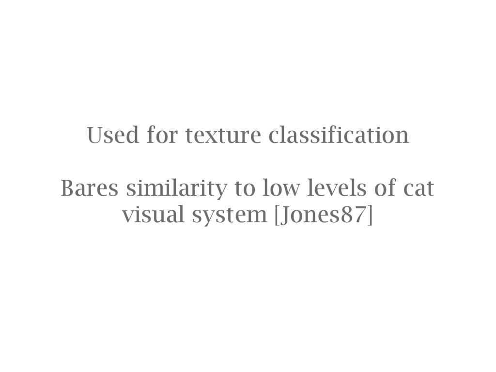
![[Jones87] Jones, J.P.; Palmer, L.A. (1987). "An evaluation of the](https://files.speakerdeck.com/presentations/50e4ae1058144e0daebfbdfd602d7e52/slide_162.jpg)
![[Krizhevsky12] Krizhevsky, Sutskever and Hinton; ImageNet Classification with Deep Convolutional](https://files.speakerdeck.com/presentations/50e4ae1058144e0daebfbdfd602d7e52/slide_163.jpg)
![[LeCun95] LeCun, Yann et. al.; Comparison of learning algorithms for](https://files.speakerdeck.com/presentations/50e4ae1058144e0daebfbdfd602d7e52/slide_164.jpg)
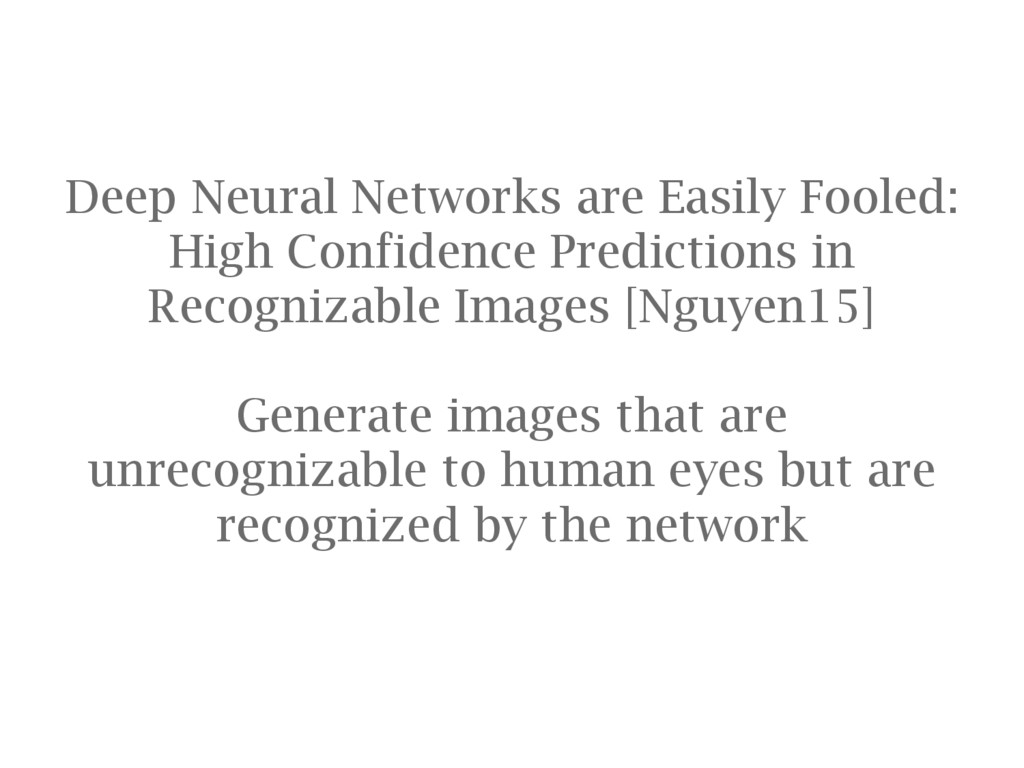
![[Nguyen15] Nguyen, Yosinski and Clune; Deep Neural Networks are Easily](https://files.speakerdeck.com/presentations/50e4ae1058144e0daebfbdfd602d7e52/slide_165.jpg)
![[Radford15] Radford, Metz, Chintala; Unsupervised Representation Learning with Deep Convolutional](https://files.speakerdeck.com/presentations/50e4ae1058144e0daebfbdfd602d7e52/slide_166.jpg)
![[Simonyan14] K. Simonyan and Zisserman; Very deep convolutional networks for](https://files.speakerdeck.com/presentations/50e4ae1058144e0daebfbdfd602d7e52/slide_167.jpg)
![[Zeiler14] Zeiler and Fergus; Visualizing and understanding convolutional networks, Computer](https://files.speakerdeck.com/presentations/50e4ae1058144e0daebfbdfd602d7e52/slide_168.jpg)