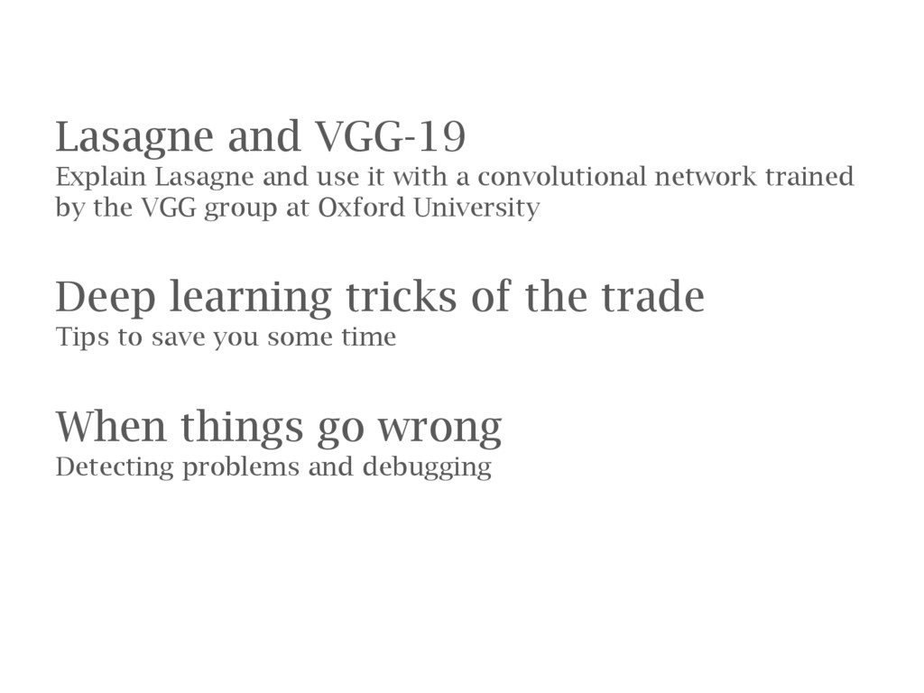
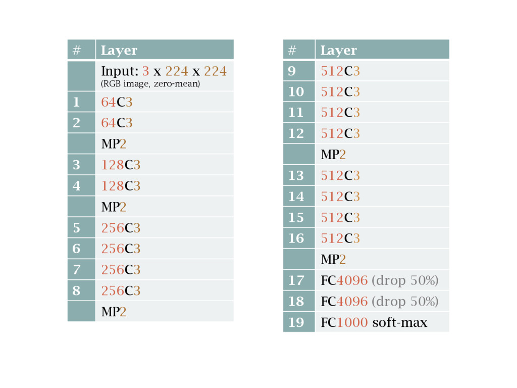
convolutional network trained by the VGG group at Oxford University Deep learning tricks of the trade Tips to save you some time When things go wrong Detecting problems and debugging
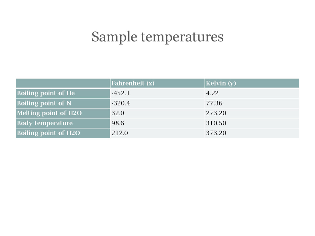
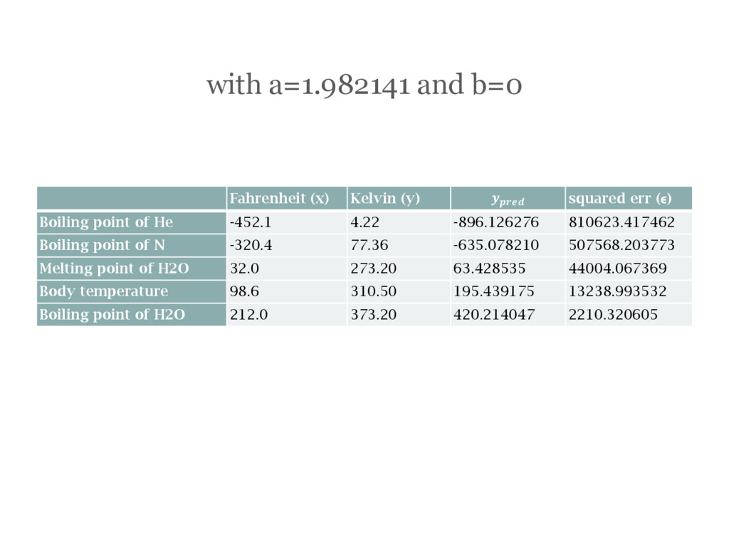
(ϵ) Boiling point of He -452.1 4.22 -896.126276 810623.417462 Boiling point of N -320.4 77.36 -635.078210 507568.203773 Melting point of H2O 32.0 273.20 63.428535 44004.067369 Body temperature 98.6 310.50 195.439175 13238.993532 Boiling point of H2O 212.0 373.20 420.214047 2210.320605
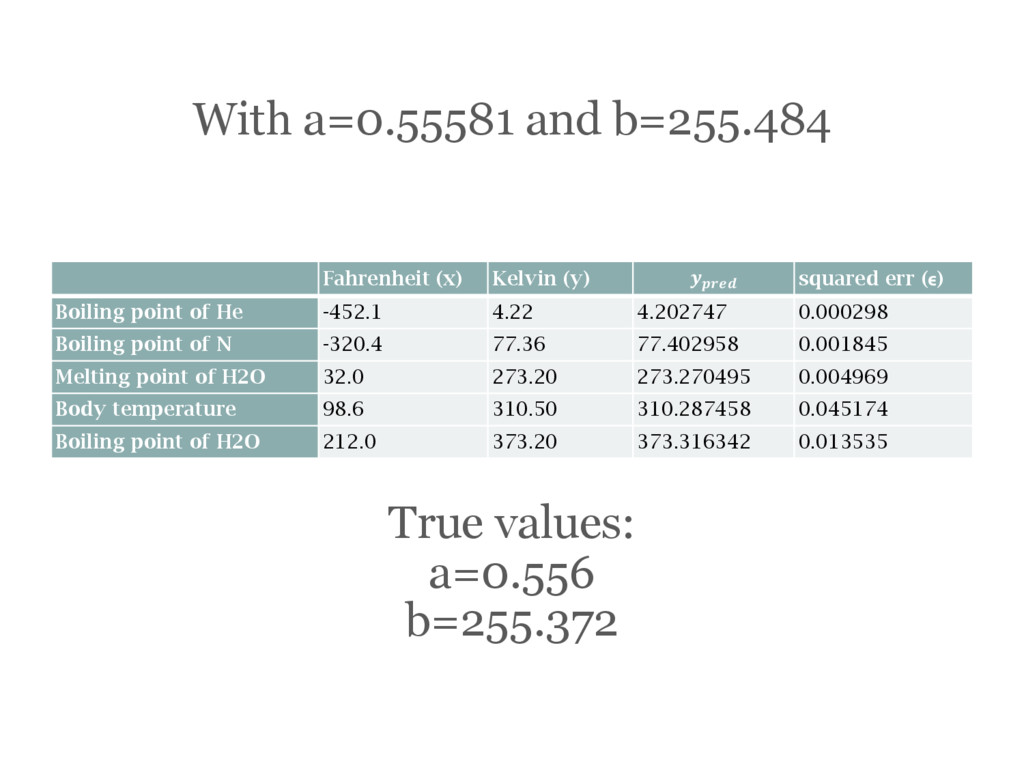
(ϵ) Boiling point of He -452.1 4.22 4.202747 0.000298 Boiling point of N -320.4 77.36 77.402958 0.001845 Melting point of H2O 32.0 273.20 273.270495 0.004969 Body temperature 98.6 310.50 310.287458 0.045174 Boiling point of H2O 212.0 373.20 373.316342 0.013535 True values: a=0.556 b=255.372
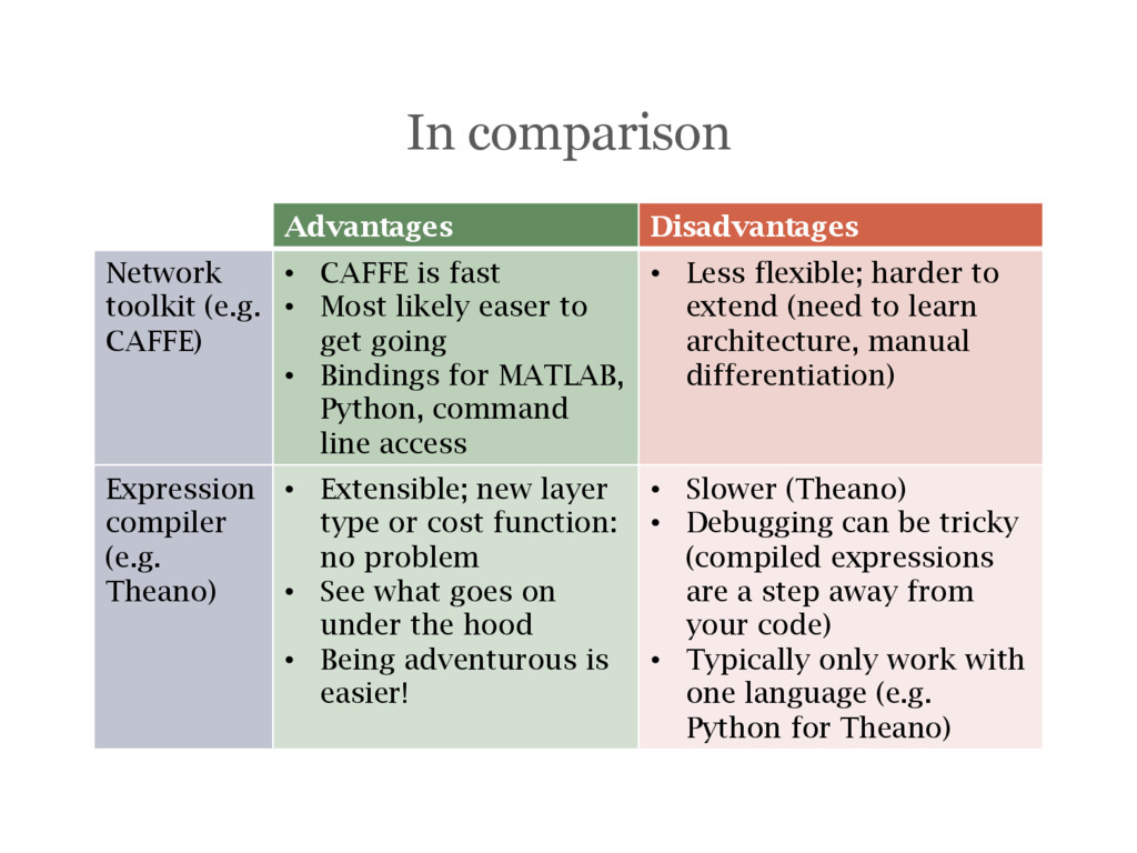
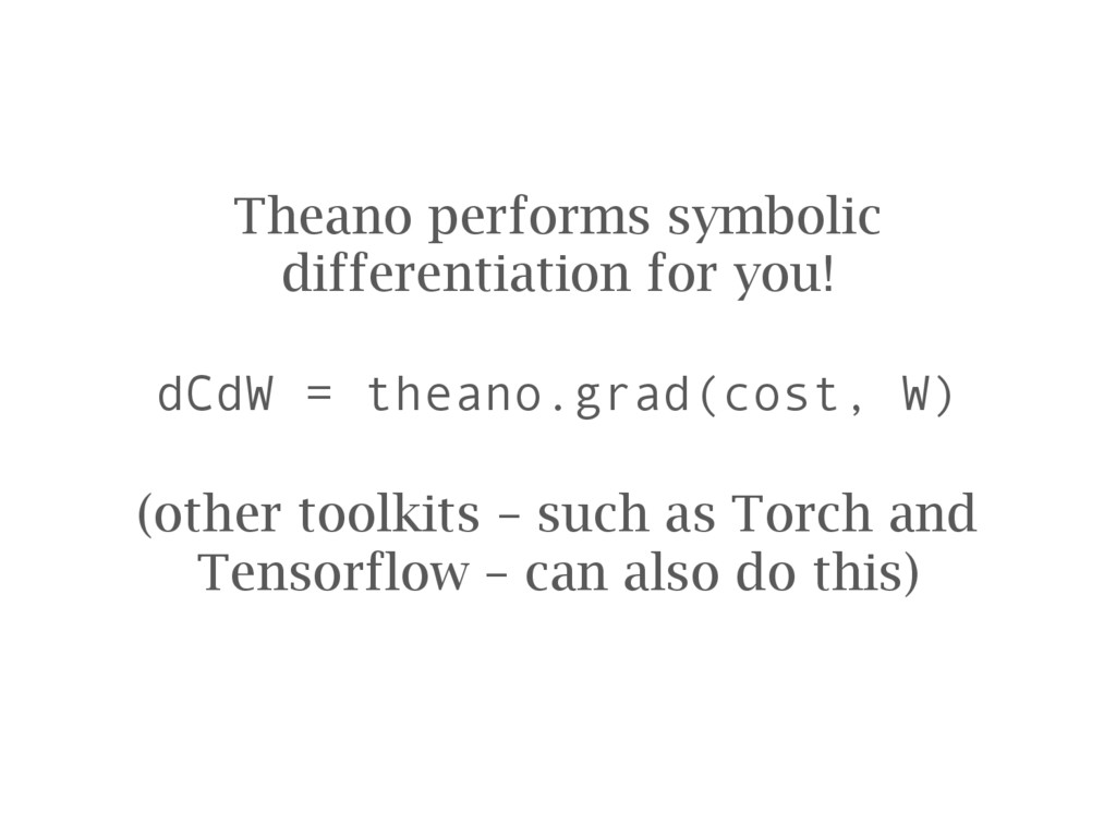
is fast • Most likely easer to get going • Bindings for MATLAB, Python, command line access • Less flexible; harder to extend (need to learn architecture, manual differentiation) Expression compiler (e.g. Theano) • Extensible; new layer type or cost function: no problem • See what goes on under the hood • Being adventurous is easier! • Slower (Theano) • Debugging can be tricky (compiled expressions are a step away from your code) • Typically only work with one language (e.g. Python for Theano)
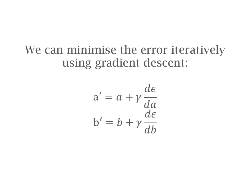
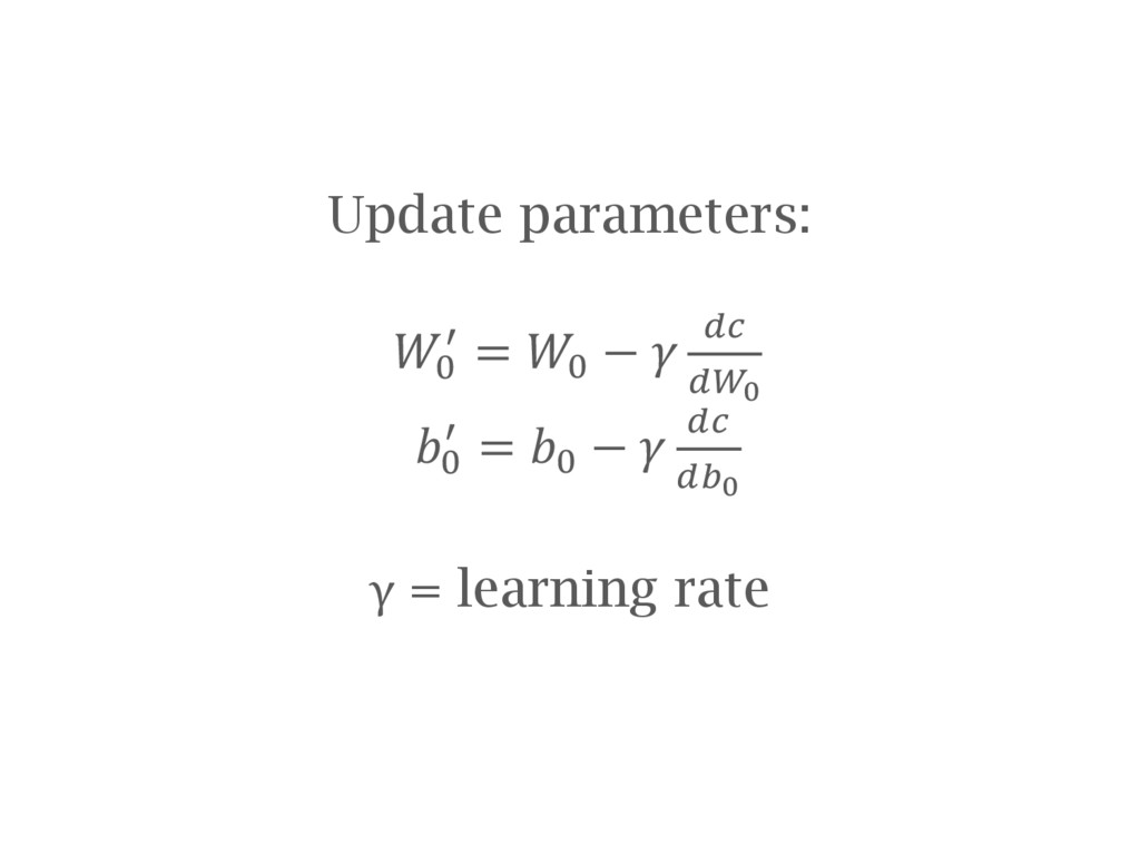
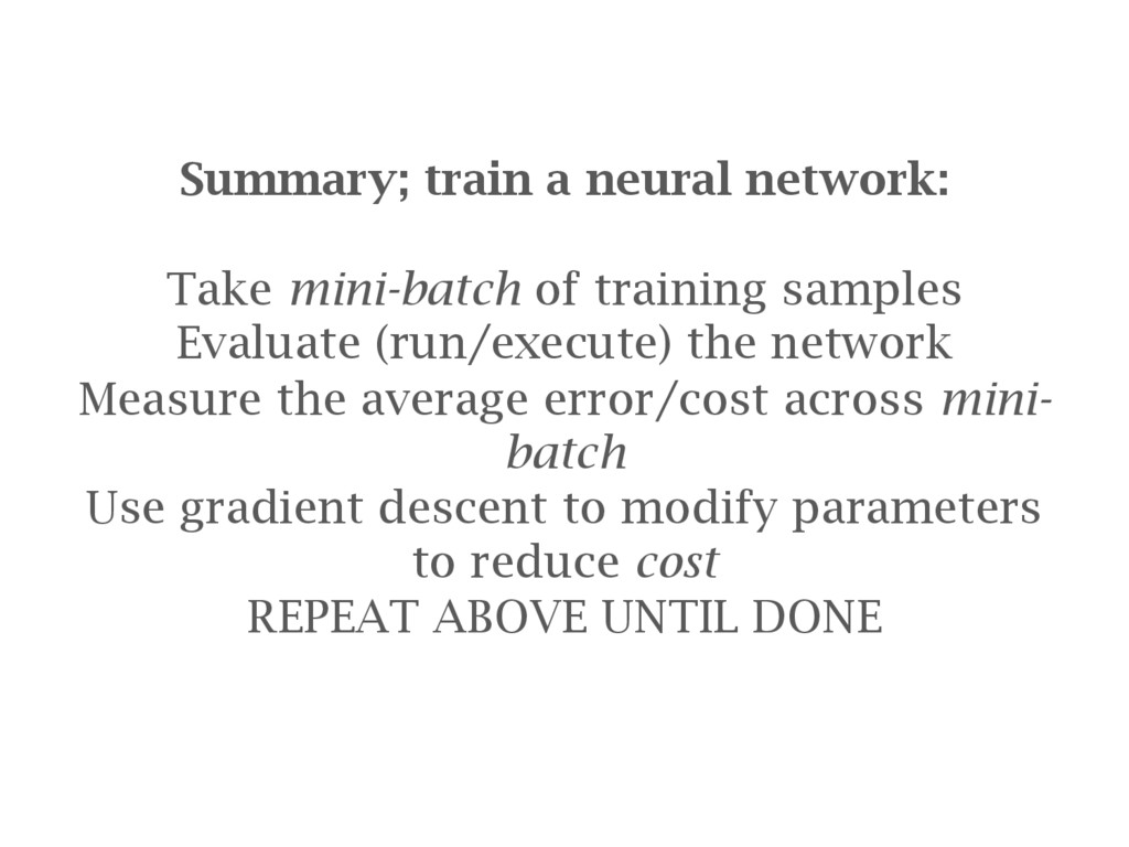
Evaluate (run/execute) the network Measure the average error/cost across mini- batch Use gradient descent to modify parameters to reduce cost REPEAT ABOVE UNTIL DONE
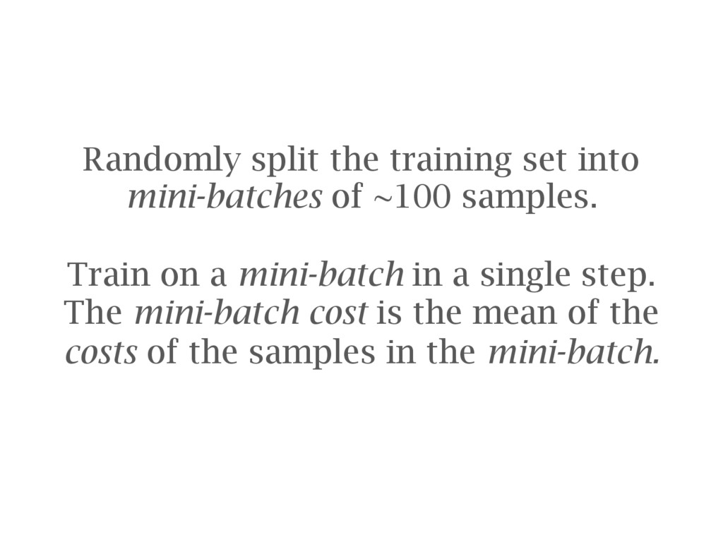
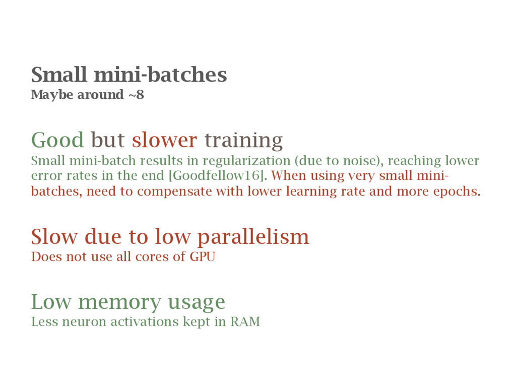
mini-batch results in regularization (due to noise), reaching lower error rates in the end [Goodfellow16]. When using very small mini- batches, need to compensate with lower learning rate and more epochs. Slow due to low parallelism Does not use all cores of GPU Low memory usage Less neuron activations kept in RAM
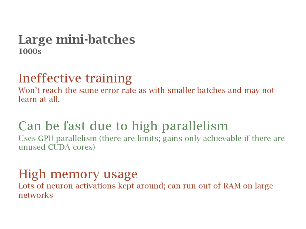
rate as with smaller batches and may not learn at all. Can be fast due to high parallelism Uses GPU parallelism (there are limits; gains only achievable if there are unused CUDA cores) High memory usage Lots of neuron activations kept around; can run out of RAM on large networks
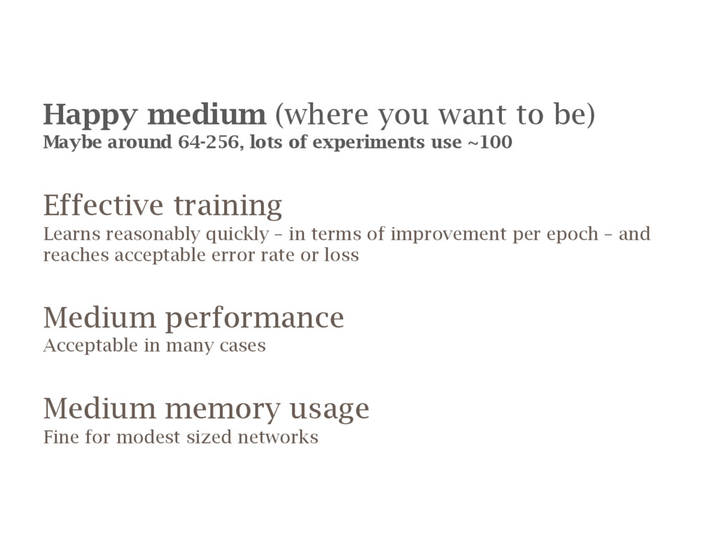
lots of experiments use ~100 Effective training Learns reasonably quickly – in terms of improvement per epoch – and reaches acceptable error rate or loss Medium performance Acceptable in many cases Medium memory usage Fine for modest sized networks
networks particularly A model over-fits when it is very good at correctly predicting samples in training set but fails to generalise to samples outside it
15] Train two networks; one given random parameters to generate an image, another to discriminate between a generated image and one from the training set
model [Simonyan14] and extract texture features from one of the convolutional layers, given a target style / painting as input Use gradient descent to iterate photo – not weights – so that its texture features match those of the target image.
![Weight initialisation [He15a] provides a good rule of thumb Most](https://files.speakerdeck.com/presentations/2efe4130ce84463cb5b7c022fc5f3725/slide_70.jpg)
![Max-pooling ‘layer’ [Ciresan12] Take maximum value from each 2 x](https://files.speakerdeck.com/presentations/2efe4130ce84463cb5b7c022fc5f3725/slide_107.jpg)
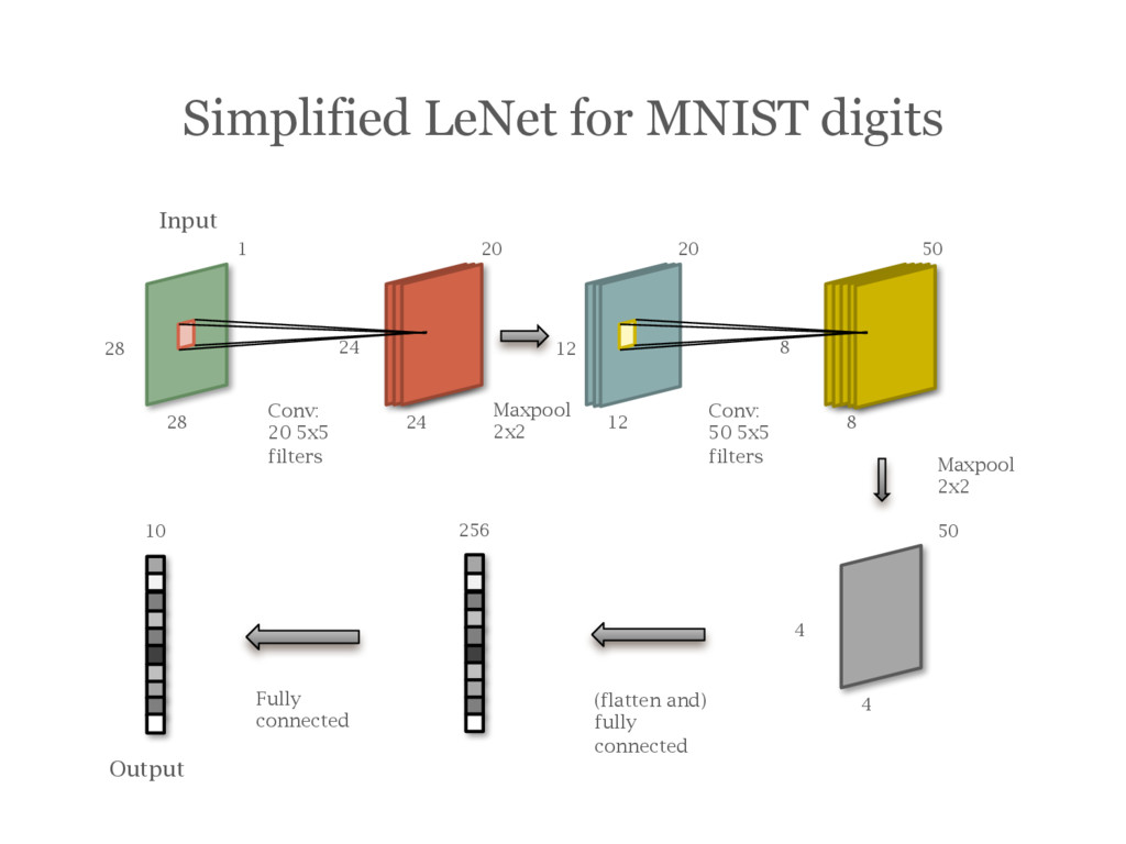
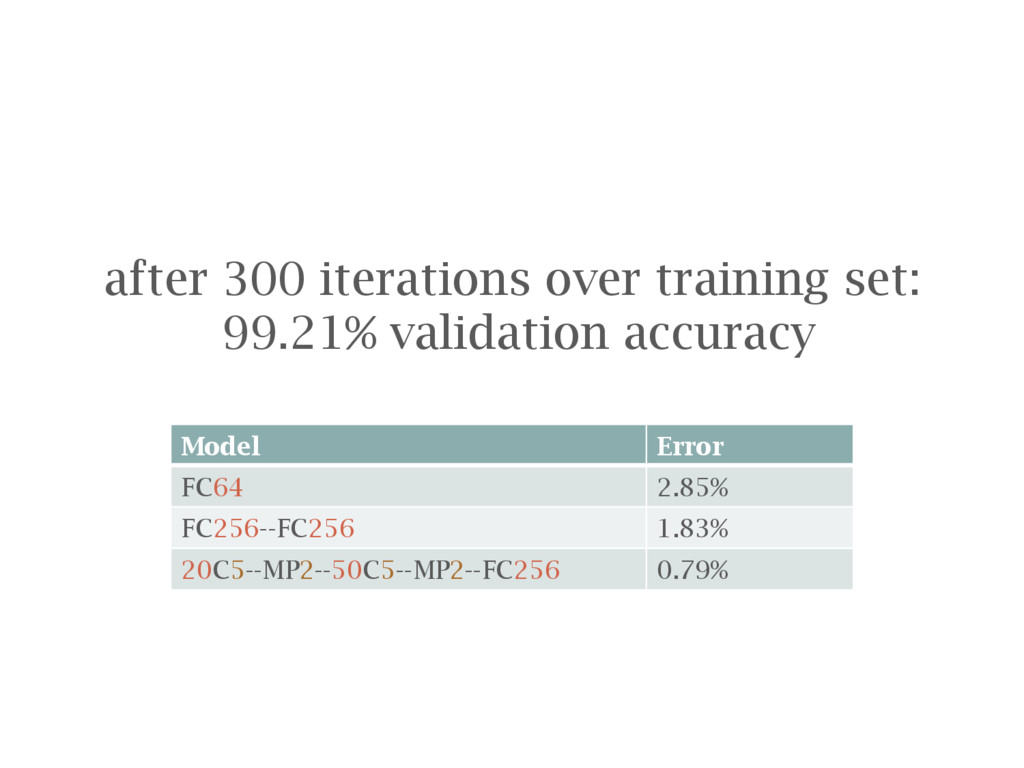
![Example: A Simplified LeNet [LeCun95] for MNIST digits](https://files.speakerdeck.com/presentations/2efe4130ce84463cb5b7c022fc5f3725/slide_109.jpg)
![What about the learned kernels? Image taken from paper [Krizhevsky12]](https://files.speakerdeck.com/presentations/2efe4130ce84463cb5b7c022fc5f3725/slide_112.jpg)
![Image taken from [Zeiler14]](https://files.speakerdeck.com/presentations/2efe4130ce84463cb5b7c022fc5f3725/slide_113.jpg)
![Image taken from [Zeiler14]](https://files.speakerdeck.com/presentations/2efe4130ce84463cb5b7c022fc5f3725/slide_114.jpg)
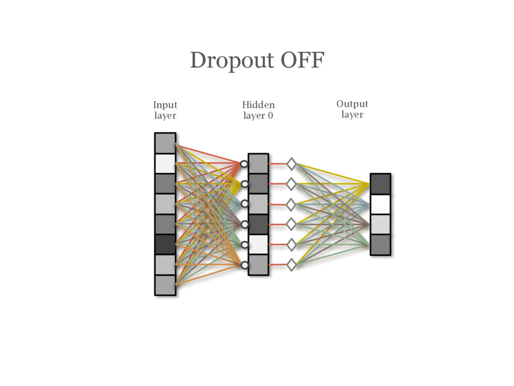
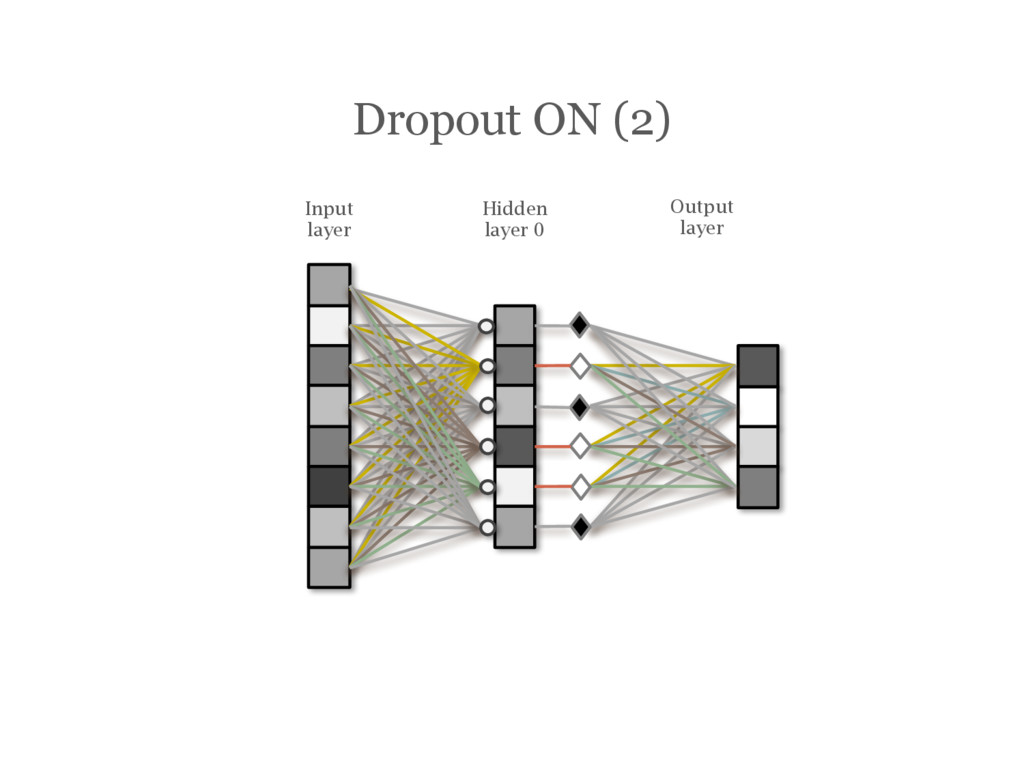
![DropOut [Hinton12] During training, randomly choose units to ‘drop out’](https://files.speakerdeck.com/presentations/2efe4130ce84463cb5b7c022fc5f3725/slide_147.jpg)
![Batch normalization [Ioffe15] is recommended in most cases Lets you](https://files.speakerdeck.com/presentations/2efe4130ce84463cb5b7c022fc5f3725/slide_156.jpg)
![Visualizing and understanding convolutional networks [Zeiler14] Visualisations of responses of](https://files.speakerdeck.com/presentations/2efe4130ce84463cb5b7c022fc5f3725/slide_212.jpg)
![Visualizing and understanding convolutional networks [Zeiler14] Image taken from [Zeiler14]](https://files.speakerdeck.com/presentations/2efe4130ce84463cb5b7c022fc5f3725/slide_213.jpg)
![Visualizing and understanding convolutional networks [Zeiler14] Image taken from [Zeiler14]](https://files.speakerdeck.com/presentations/2efe4130ce84463cb5b7c022fc5f3725/slide_214.jpg)
![Learning to generate chairs with convolutional neural networks [Dosovitskiy15] Network](https://files.speakerdeck.com/presentations/2efe4130ce84463cb5b7c022fc5f3725/slide_217.jpg)
![Learning to generate chairs with convolutional neural networks [Dosovitskiy15] Image](https://files.speakerdeck.com/presentations/2efe4130ce84463cb5b7c022fc5f3725/slide_218.jpg)
![Generative Adversarial Nets [Radford15] Images of bedrooms generated using neural](https://files.speakerdeck.com/presentations/2efe4130ce84463cb5b7c022fc5f3725/slide_220.jpg)
![Generative Adversarial Nets [Radford15] Image taken from [Radford15]](https://files.speakerdeck.com/presentations/2efe4130ce84463cb5b7c022fc5f3725/slide_221.jpg)
![A Neural Algorithm of Artistic Style [Gatys15] Take an OxfordNet](https://files.speakerdeck.com/presentations/2efe4130ce84463cb5b7c022fc5f3725/slide_222.jpg)
![A Neural Algorithm of Artistic Style [Gatys15] Image taken from](https://files.speakerdeck.com/presentations/2efe4130ce84463cb5b7c022fc5f3725/slide_223.jpg)
![[Dosovitskiy15] Dosovitskiy, Springenberg and Box; Learning to generate chairs with](https://files.speakerdeck.com/presentations/2efe4130ce84463cb5b7c022fc5f3725/slide_227.jpg)
![[Gatys15] Gatys, Echer, Bethge; A Neural Algorithm of Artistic Style,](https://files.speakerdeck.com/presentations/2efe4130ce84463cb5b7c022fc5f3725/slide_228.jpg)
![[He15a] He, Zhang, Ren and Sun; Delving Deep into Rectifiers:](https://files.speakerdeck.com/presentations/2efe4130ce84463cb5b7c022fc5f3725/slide_229.jpg)
![[He15b] He, Kaiming, et al. "Deep Residual Learning for Image](https://files.speakerdeck.com/presentations/2efe4130ce84463cb5b7c022fc5f3725/slide_230.jpg)
![[Hinton12] G.E. Hinton, N. Srivastava, A. Krizhevsky, I. Sutskever and](https://files.speakerdeck.com/presentations/2efe4130ce84463cb5b7c022fc5f3725/slide_231.jpg)
![[Ioffe15] Ioffe, S.; Szegedy C.. (2015). “Batch Normalization: Accelerating Deep](https://files.speakerdeck.com/presentations/2efe4130ce84463cb5b7c022fc5f3725/slide_232.jpg)
![[Radford15] Radford, Metz, Chintala; Unsupervised Representation Learning with Deep Convolutional](https://files.speakerdeck.com/presentations/2efe4130ce84463cb5b7c022fc5f3725/slide_233.jpg)
![[Simonyan14] K. Simonyan and Zisserman; Very deep convolutional networks for](https://files.speakerdeck.com/presentations/2efe4130ce84463cb5b7c022fc5f3725/slide_234.jpg)
![[Wang14] Wang, Dan, and Yi Shang. "A new active labeling](https://files.speakerdeck.com/presentations/2efe4130ce84463cb5b7c022fc5f3725/slide_235.jpg)
![[Zeiler14] Zeiler and Fergus; Visualizing and understanding convolutional networks, Computer](https://files.speakerdeck.com/presentations/2efe4130ce84463cb5b7c022fc5f3725/slide_236.jpg)