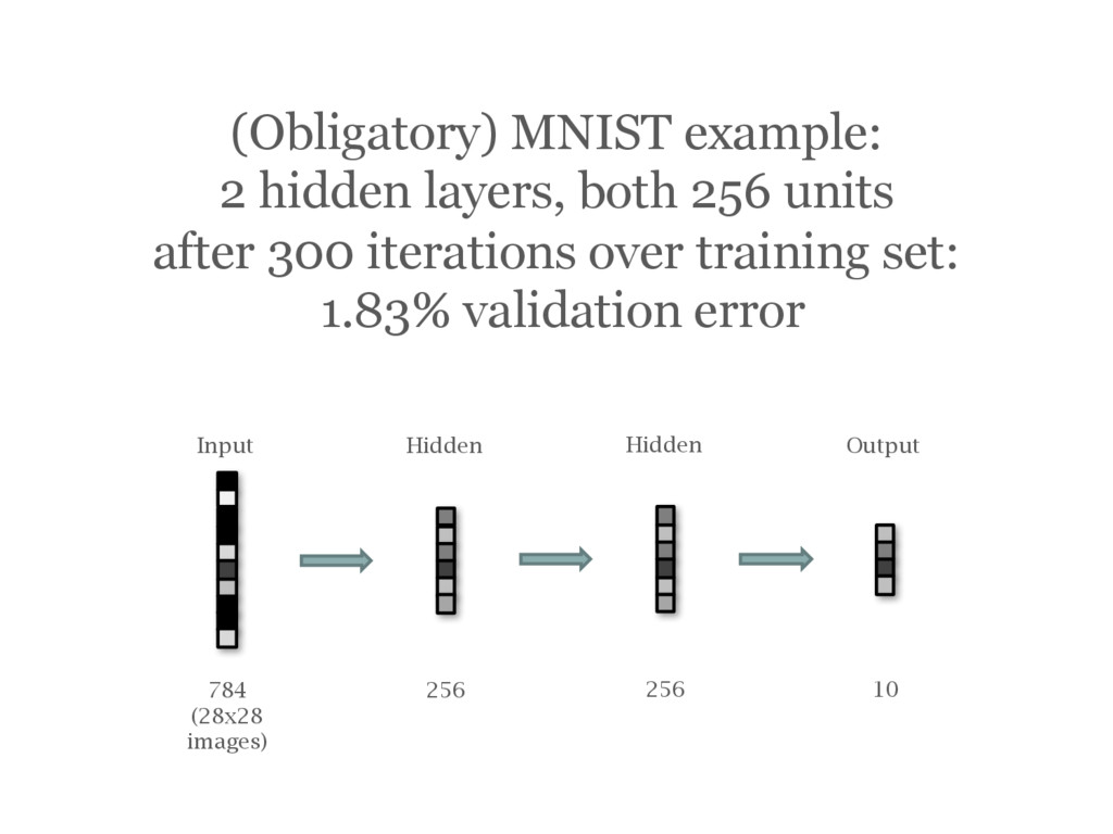
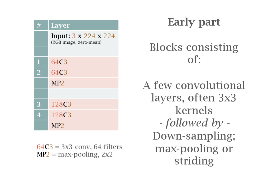
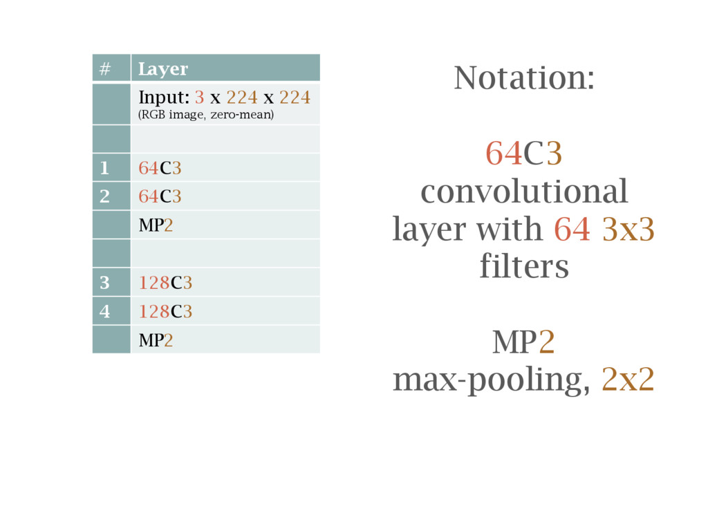
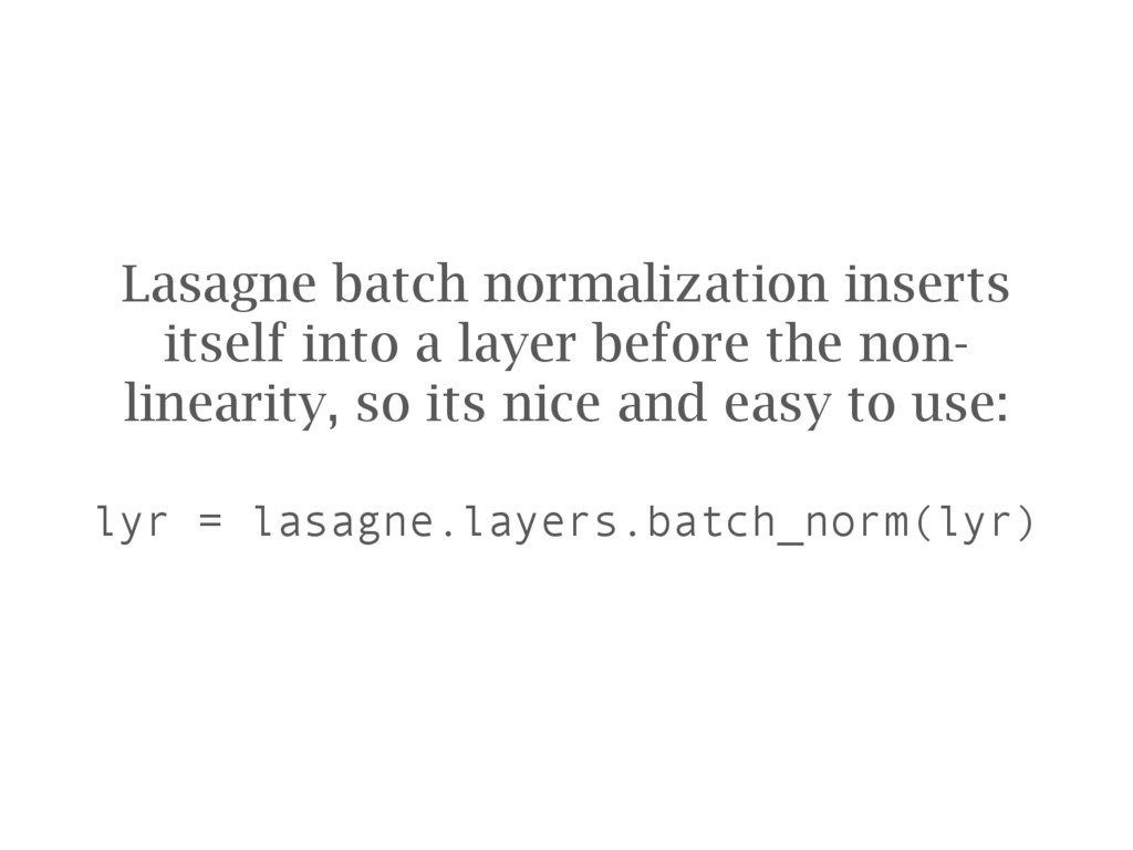
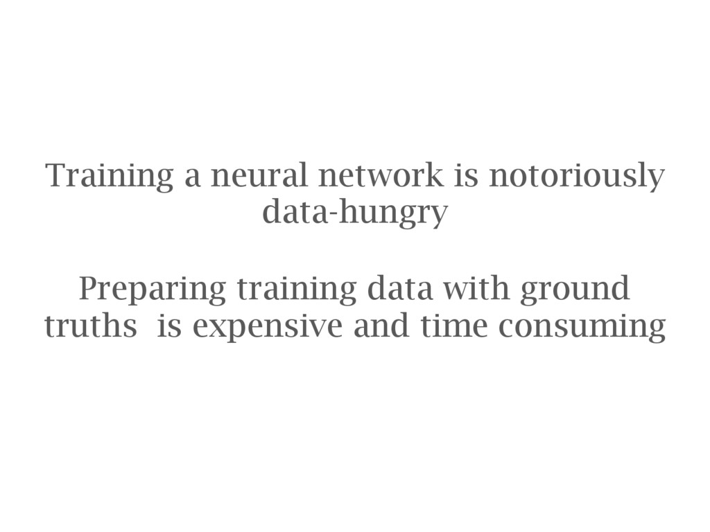
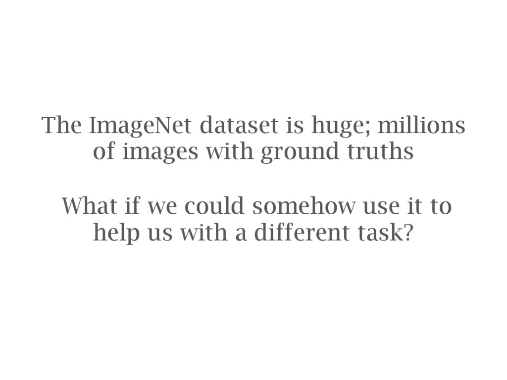
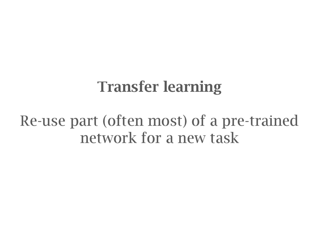
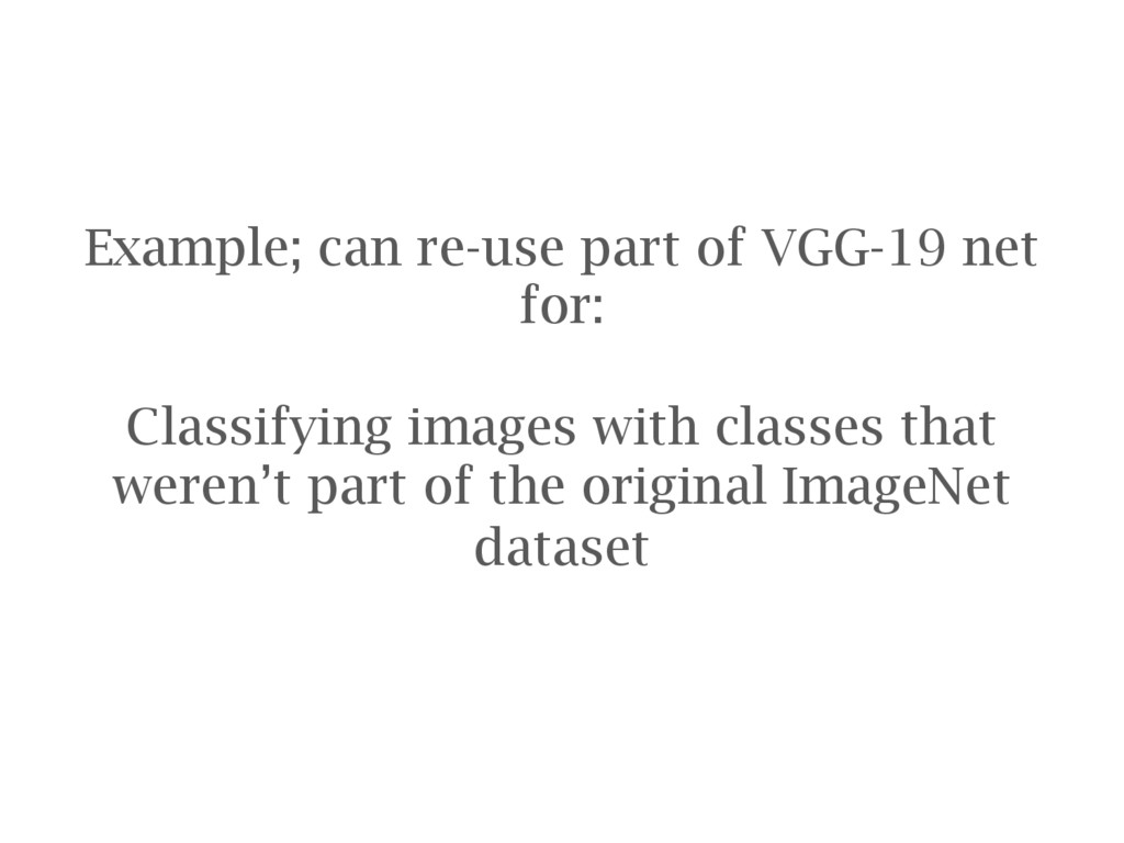
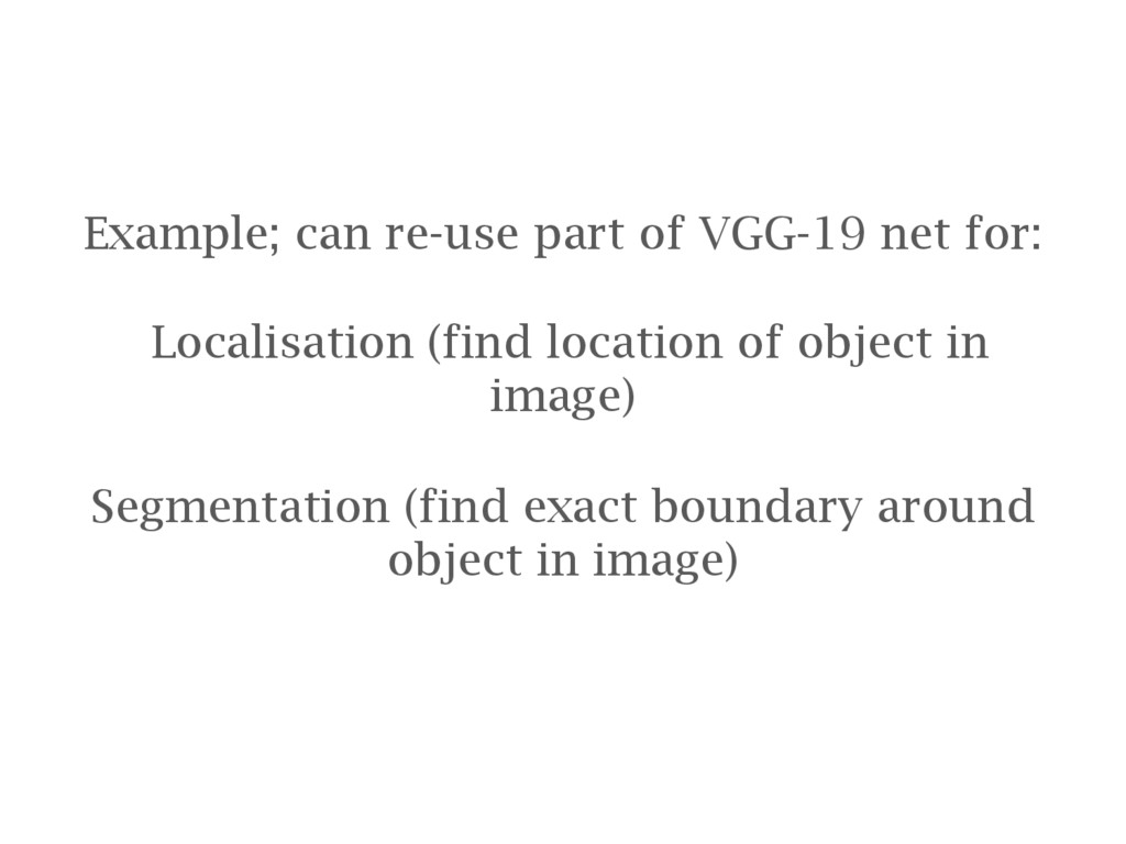
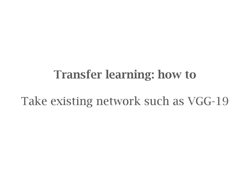
networks A few tips on building and training neural networks OxfordNet / VGG and transfer learning Using a convolutional network trained by the VGG group at Oxford University and re-purposing it for your needs
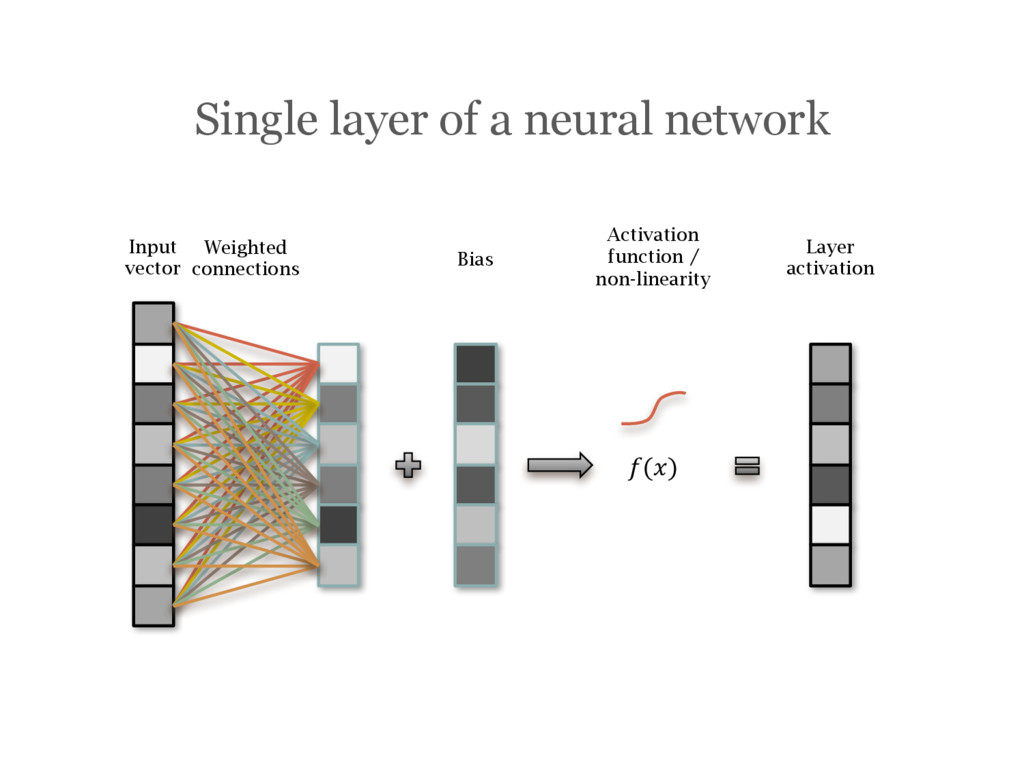
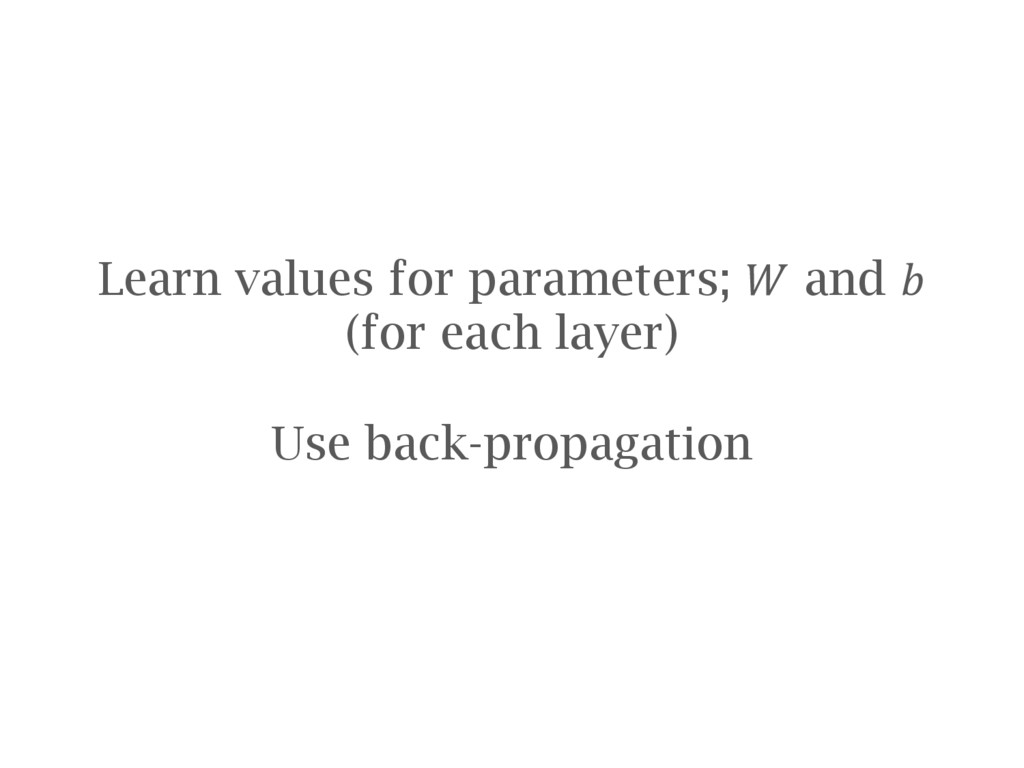
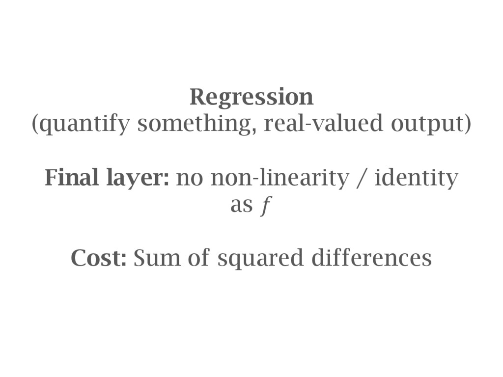
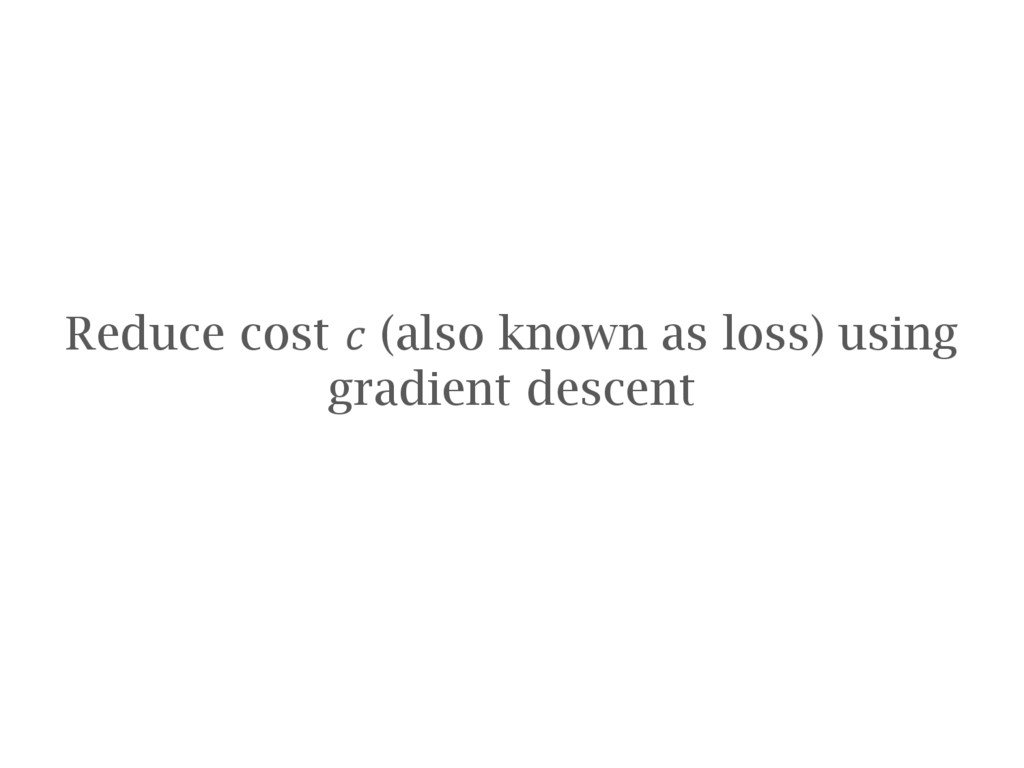
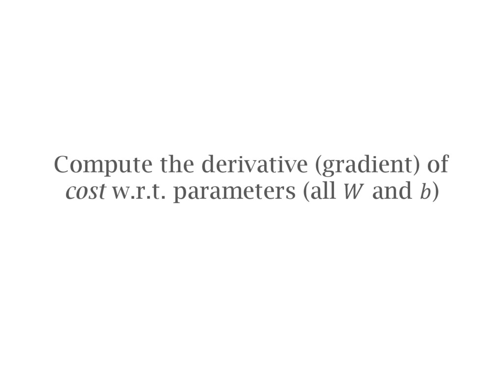
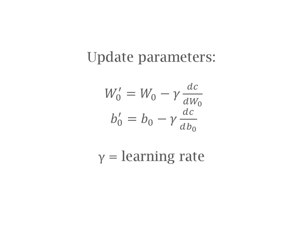
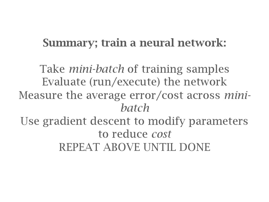
Evaluate (run/execute) the network Measure the average error/cost across mini- batch Use gradient descent to modify parameters to reduce cost REPEAT ABOVE UNTIL DONE
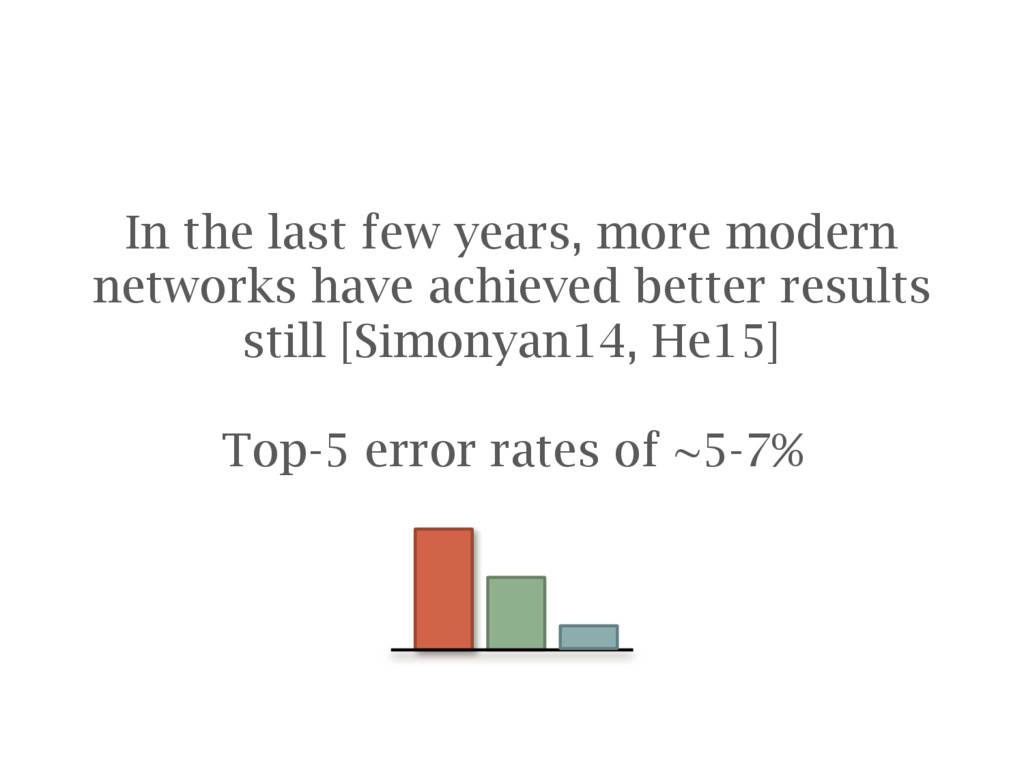
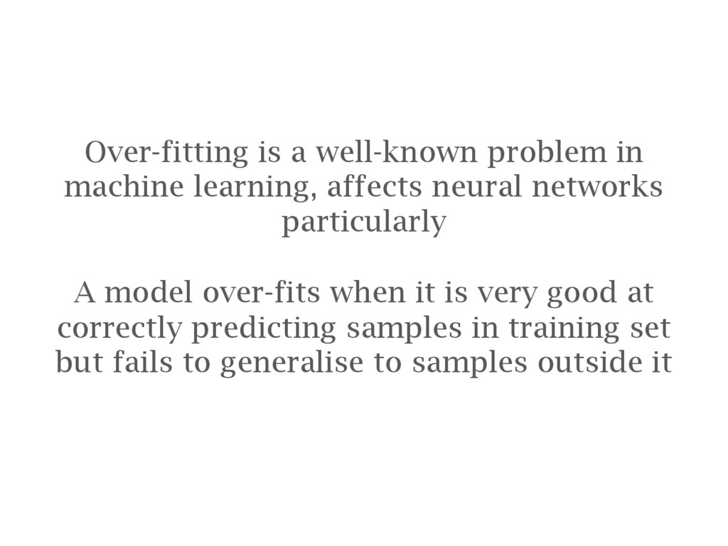
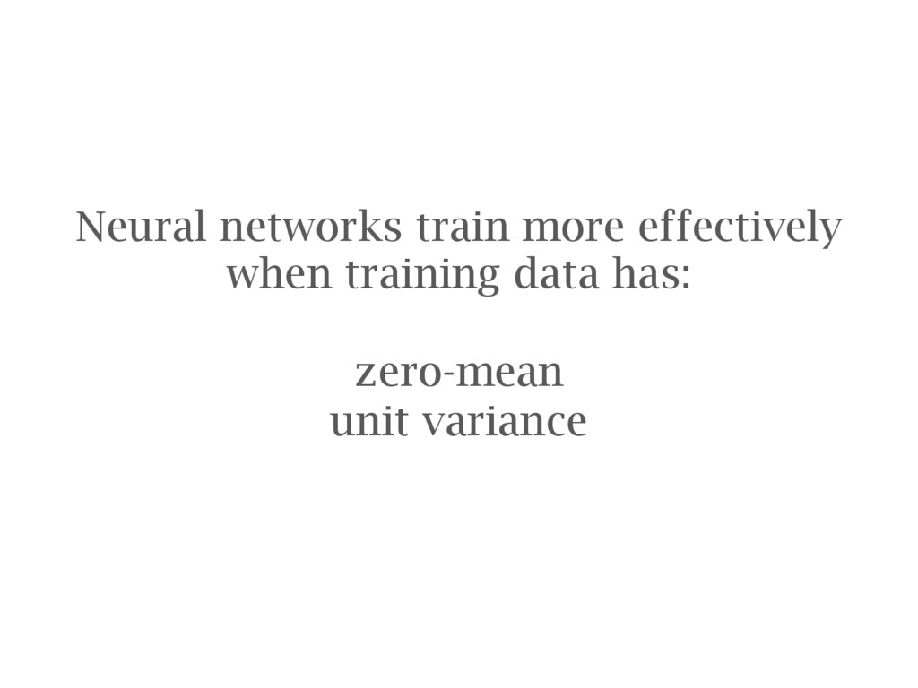
networks particularly A model over-fits when it is very good at correctly predicting samples in training set but fails to generalise to samples outside it
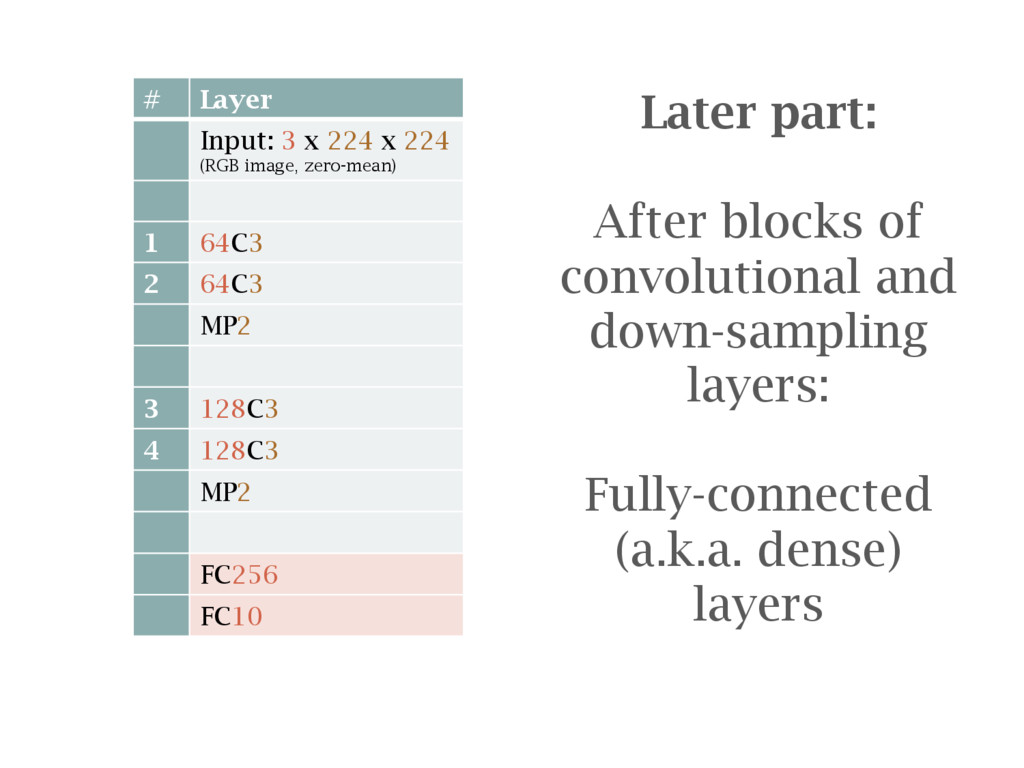
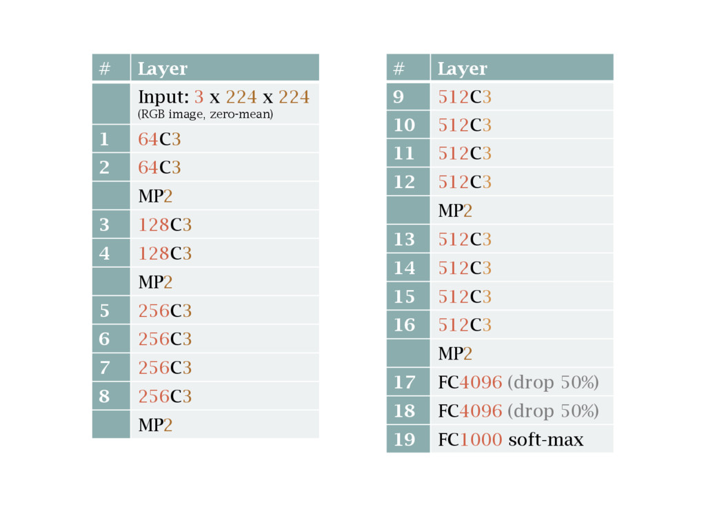
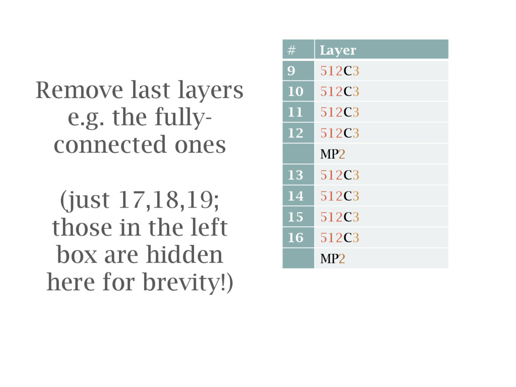
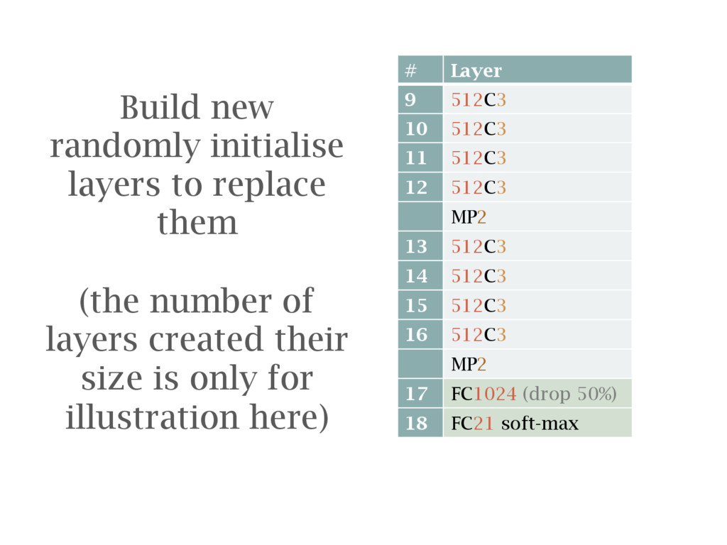
MP2 13 512C3 14 512C3 15 512C3 16 512C3 MP2 Remove last layers e.g. the fully- connected ones (just 17,18,19; those in the left box are hidden here for brevity!)
MP2 13 512C3 14 512C3 15 512C3 16 512C3 MP2 17 FC1024 (drop 50%) 18 FC21 soft-max Build new randomly initialise layers to replace them (the number of layers created their size is only for illustration here)
model [Simonyan14] and extract texture features from one of the convolutional layers, given a target style / painting as input Use gradient descent to iterate photo – not weights – so that its texture features match those of the target image.
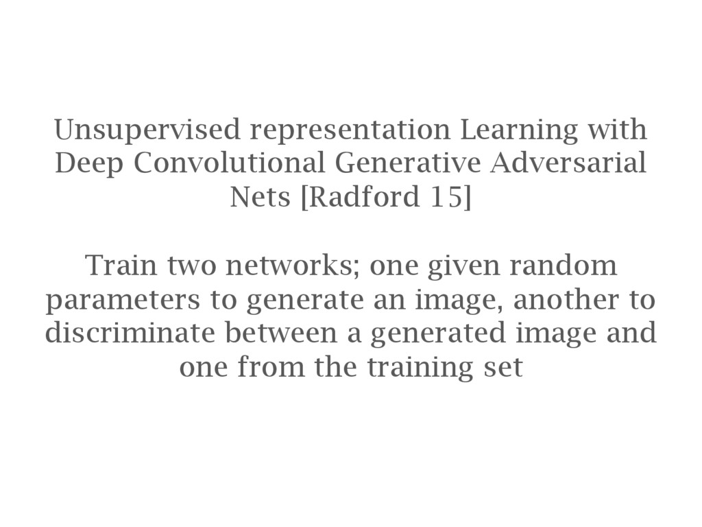
15] Train two networks; one given random parameters to generate an image, another to discriminate between a generated image and one from the training set
![Down-sampling: max-pooling ‘layer’ [Ciresan12] Take maximum value from each 2](https://files.speakerdeck.com/presentations/3acbc1c8f3d14eba8d6eaa166eeb1cda/slide_74.jpg)
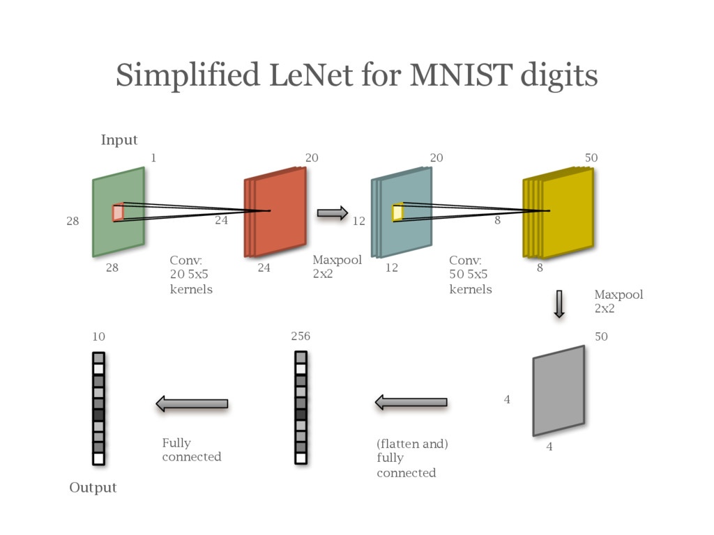
![Example: A Simplified LeNet [LeCun95] for MNIST digits](https://files.speakerdeck.com/presentations/3acbc1c8f3d14eba8d6eaa166eeb1cda/slide_76.jpg)
![What about the learned kernels? Image taken from paper [Krizhevsky12]](https://files.speakerdeck.com/presentations/3acbc1c8f3d14eba8d6eaa166eeb1cda/slide_79.jpg)
![Image taken from [Zeiler14]](https://files.speakerdeck.com/presentations/3acbc1c8f3d14eba8d6eaa166eeb1cda/slide_80.jpg)
![Image taken from [Zeiler14]](https://files.speakerdeck.com/presentations/3acbc1c8f3d14eba8d6eaa166eeb1cda/slide_81.jpg)
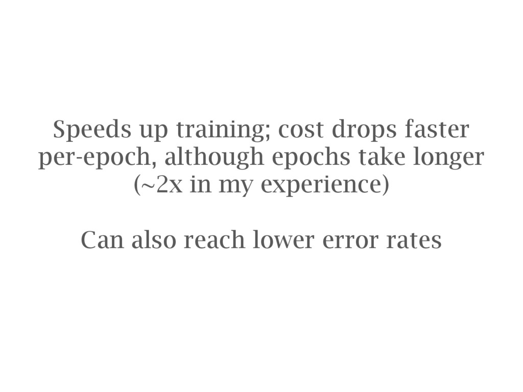
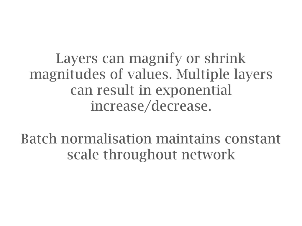
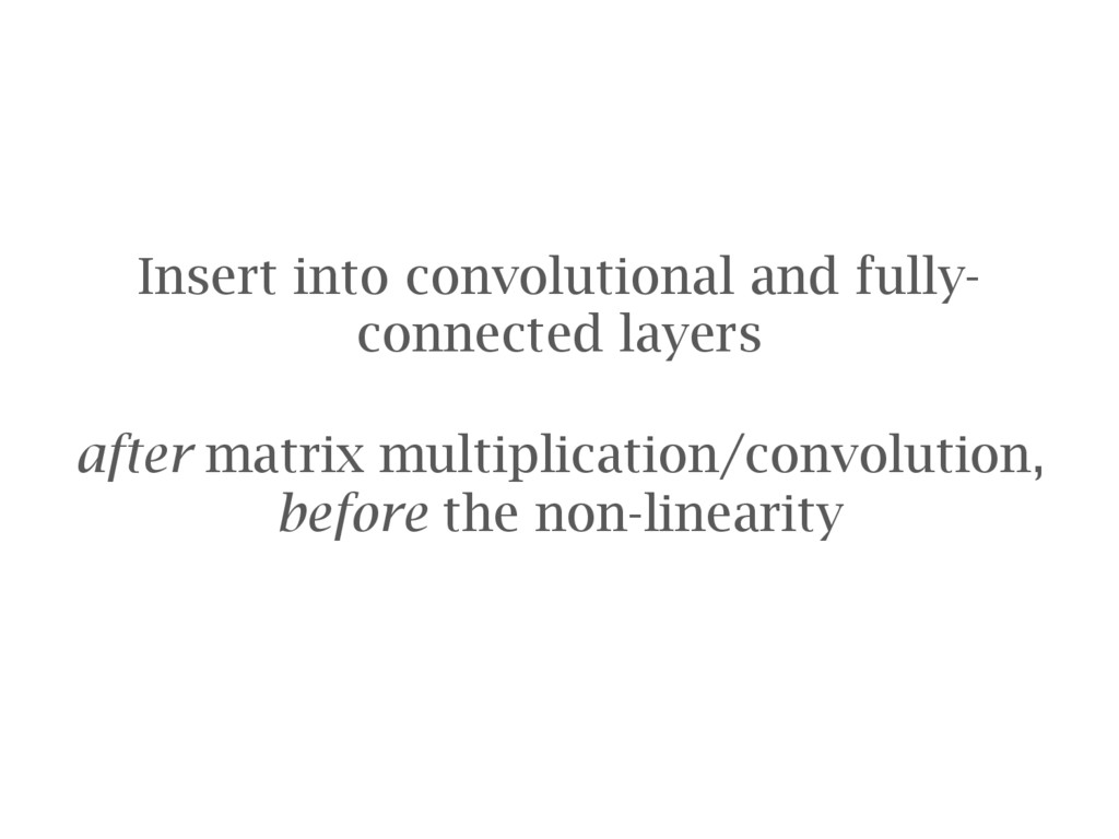
![Batch normalization [Ioffe15] is recommended in most cases Necessary for](https://files.speakerdeck.com/presentations/3acbc1c8f3d14eba8d6eaa166eeb1cda/slide_99.jpg)
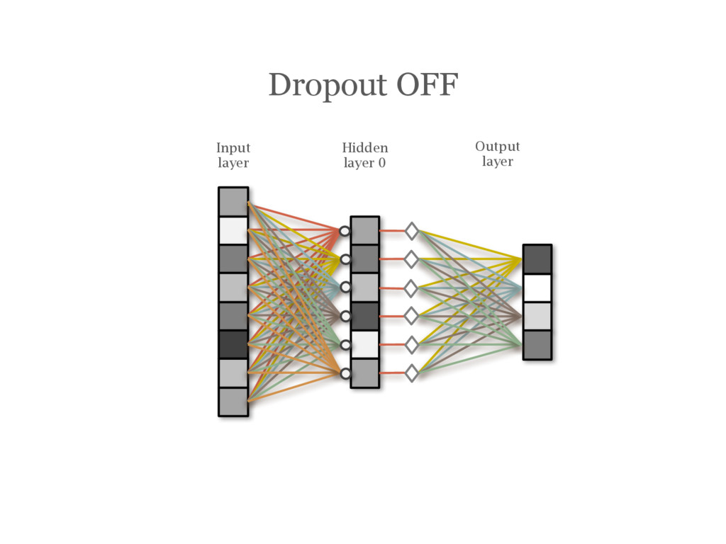
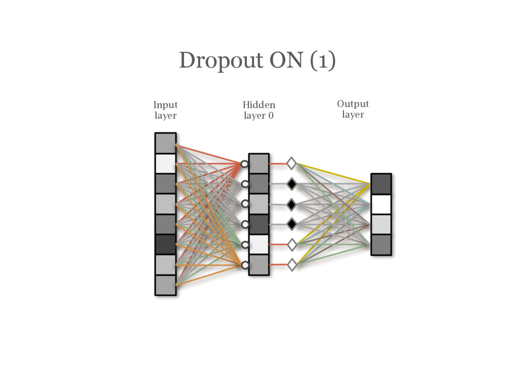
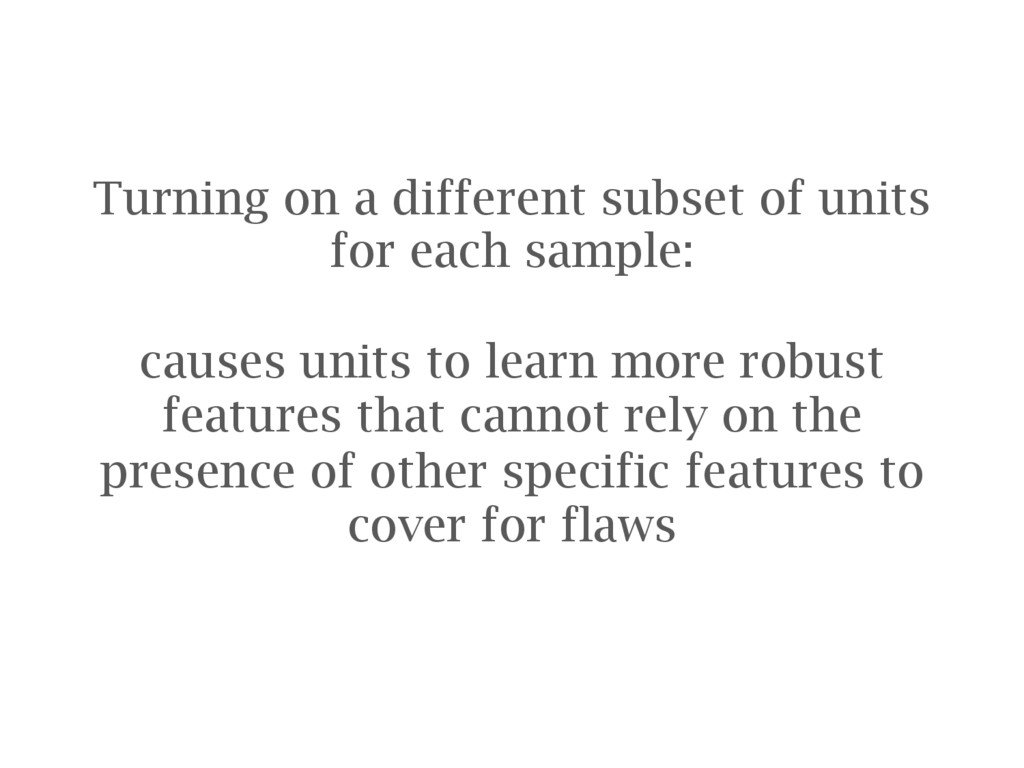
![DropOut [Hinton12] During training, randomly choose units to ‘drop out’](https://files.speakerdeck.com/presentations/3acbc1c8f3d14eba8d6eaa166eeb1cda/slide_107.jpg)
![Visualizing and understanding convolutional networks [Zeiler14] Visualisations of responses of](https://files.speakerdeck.com/presentations/3acbc1c8f3d14eba8d6eaa166eeb1cda/slide_162.jpg)
![Visualizing and understanding convolutional networks [Zeiler14] Image taken from [Zeiler14]](https://files.speakerdeck.com/presentations/3acbc1c8f3d14eba8d6eaa166eeb1cda/slide_163.jpg)
![Visualizing and understanding convolutional networks [Zeiler14] Image taken from [Zeiler14]](https://files.speakerdeck.com/presentations/3acbc1c8f3d14eba8d6eaa166eeb1cda/slide_164.jpg)
![Learning to generate chairs with convolutional neural networks [Dosovitskiy15] Network](https://files.speakerdeck.com/presentations/3acbc1c8f3d14eba8d6eaa166eeb1cda/slide_167.jpg)
![Learning to generate chairs with convolutional neural networks [Dosovitskiy15] Image](https://files.speakerdeck.com/presentations/3acbc1c8f3d14eba8d6eaa166eeb1cda/slide_168.jpg)
![A Neural Algorithm of Artistic Style [Gatys15] Take an OxfordNet](https://files.speakerdeck.com/presentations/3acbc1c8f3d14eba8d6eaa166eeb1cda/slide_169.jpg)
![A Neural Algorithm of Artistic Style [Gatys15] Image taken from](https://files.speakerdeck.com/presentations/3acbc1c8f3d14eba8d6eaa166eeb1cda/slide_170.jpg)
![Generative Adversarial Nets [Radford15] Images of bedrooms generated using neural](https://files.speakerdeck.com/presentations/3acbc1c8f3d14eba8d6eaa166eeb1cda/slide_172.jpg)
![Generative Adversarial Nets [Radford15] Image taken from [Radford15]](https://files.speakerdeck.com/presentations/3acbc1c8f3d14eba8d6eaa166eeb1cda/slide_173.jpg)
![[Dosovitskiy15] Dosovitskiy, Springenberg and Box; Learning to generate chairs with](https://files.speakerdeck.com/presentations/3acbc1c8f3d14eba8d6eaa166eeb1cda/slide_177.jpg)
![[Gatys15] Gatys, Echer, Bethge; A Neural Algorithm of Artistic Style,](https://files.speakerdeck.com/presentations/3acbc1c8f3d14eba8d6eaa166eeb1cda/slide_178.jpg)
![[He15a] He, Zhang, Ren and Sun; Delving Deep into Rectifiers:](https://files.speakerdeck.com/presentations/3acbc1c8f3d14eba8d6eaa166eeb1cda/slide_179.jpg)
![[He15b] He, Kaiming, et al. "Deep Residual Learning for Image](https://files.speakerdeck.com/presentations/3acbc1c8f3d14eba8d6eaa166eeb1cda/slide_180.jpg)
![[Hinton12] G.E. Hinton, N. Srivastava, A. Krizhevsky, I. Sutskever and](https://files.speakerdeck.com/presentations/3acbc1c8f3d14eba8d6eaa166eeb1cda/slide_181.jpg)
![[Ioffe15] Ioffe, S.; Szegedy C.. (2015). “Batch Normalization: Accelerating Deep](https://files.speakerdeck.com/presentations/3acbc1c8f3d14eba8d6eaa166eeb1cda/slide_182.jpg)
![[Jones87] Jones, J.P.; Palmer, L.A. (1987). "An evaluation of the](https://files.speakerdeck.com/presentations/3acbc1c8f3d14eba8d6eaa166eeb1cda/slide_183.jpg)
![[Lin13] Lin, Min, Qiang Chen, and Shuicheng Yan. "Network in](https://files.speakerdeck.com/presentations/3acbc1c8f3d14eba8d6eaa166eeb1cda/slide_184.jpg)
![[Nesterov83] Nesterov, Y. A method of solving a convex programming](https://files.speakerdeck.com/presentations/3acbc1c8f3d14eba8d6eaa166eeb1cda/slide_185.jpg)
![[Radford15] Radford, Metz, Chintala; Unsupervised Representation Learning with Deep Convolutional](https://files.speakerdeck.com/presentations/3acbc1c8f3d14eba8d6eaa166eeb1cda/slide_186.jpg)
![[Sutskever13] Sutskever, Ilya, et al. On the importance of initialization](https://files.speakerdeck.com/presentations/3acbc1c8f3d14eba8d6eaa166eeb1cda/slide_187.jpg)
![[Simonyan14] K. Simonyan and Zisserman; Very deep convolutional networks for](https://files.speakerdeck.com/presentations/3acbc1c8f3d14eba8d6eaa166eeb1cda/slide_188.jpg)
![[Wang14] Wang, Dan, and Yi Shang. "A new active labeling](https://files.speakerdeck.com/presentations/3acbc1c8f3d14eba8d6eaa166eeb1cda/slide_189.jpg)
![[Zeiler14] Zeiler and Fergus; Visualizing and understanding convolutional networks, Computer](https://files.speakerdeck.com/presentations/3acbc1c8f3d14eba8d6eaa166eeb1cda/slide_190.jpg)