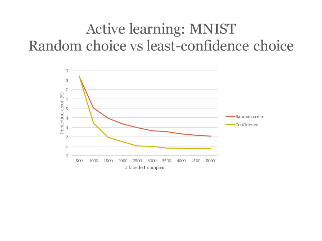
convolutional network trained by the VGG group at Oxford University Deep learning tricks of the trade tips to save you some time Active learning less training data by careful choice
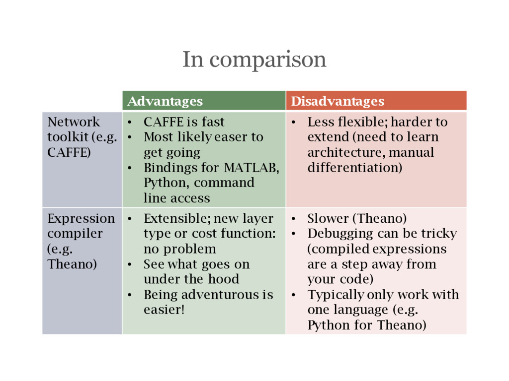
is fast • Most likely easer to get going • Bindings for MATLAB, Python, command line access • Less flexible; harder to extend (need to learn architecture, manual differentiation) Expression compiler (e.g. Theano) • Extensible; new layer type or cost function: no problem • See what goes on under the hood • Being adventurous is easier! • Slower (Theano) • Debugging can be tricky (compiled expressions are a step away from your code) • Typically only work with one language (e.g. Python for Theano)
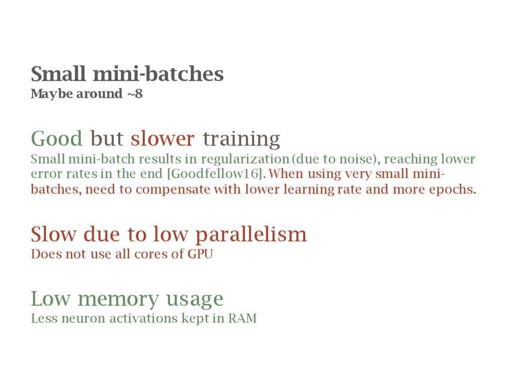
mini-batch results in regularization (due to noise), reaching lower error rates in the end [Goodfellow16]. When using very small mini- batches, need to compensate with lower learning rate and more epochs. Slow due to low parallelism Does not use all cores of GPU Low memory usage Less neuron activations kept in RAM
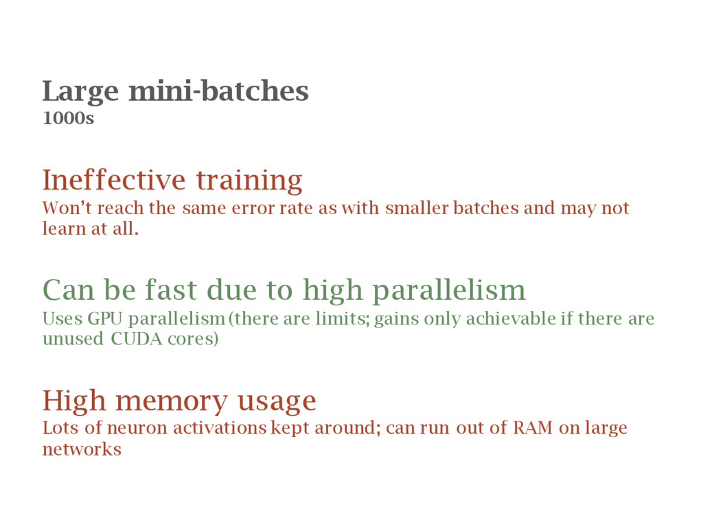
rate as with smaller batches and may not learn at all. Can be fast due to high parallelism Uses GPU parallelism (there are limits; gains only achievable if there are unused CUDA cores) High memory usage Lots of neuron activations kept around; can run out of RAM on large networks
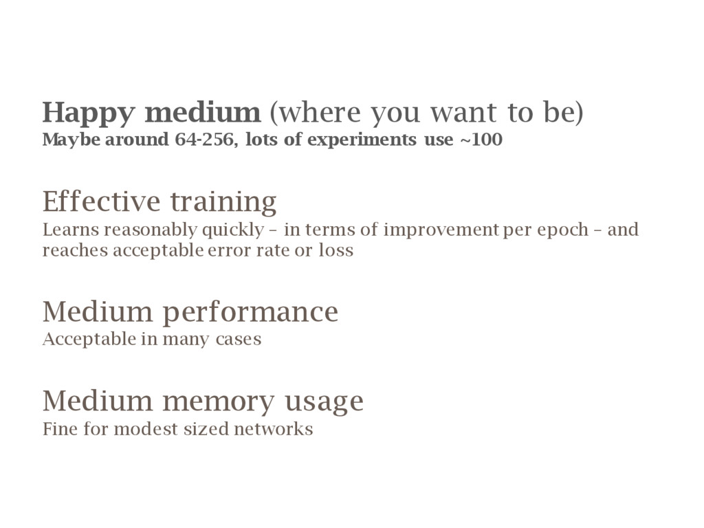
lots of experiments use ~100 Effective training Learns reasonably quickly – in terms of improvement per epoch – and reaches acceptable error rate or loss Medium performance Acceptable in many cases Medium memory usage Fine for modest sized networks
![Max-pooling ‘layer’ [Ciresan12] Take maximum value from each 2 x](https://files.speakerdeck.com/presentations/48b8e5fab208446fae0cc8bea631da6a/slide_45.jpg)
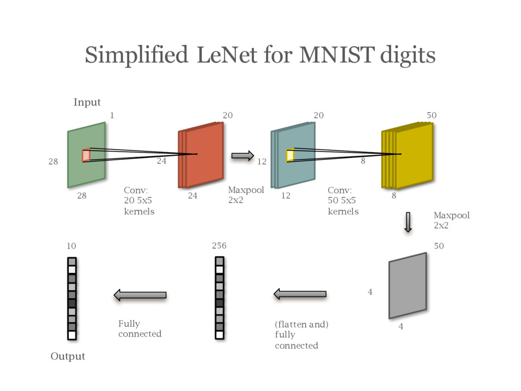
![Example: A Simplified LeNet [LeCun95] for MNIST digits](https://files.speakerdeck.com/presentations/48b8e5fab208446fae0cc8bea631da6a/slide_46.jpg)
![Batch normalization [Ioffe15] is recommended in most cases Speeds up](https://files.speakerdeck.com/presentations/48b8e5fab208446fae0cc8bea631da6a/slide_86.jpg)
![Can be partially addressed with careful weight initialization [He15]. Batch](https://files.speakerdeck.com/presentations/48b8e5fab208446fae0cc8bea631da6a/slide_92.jpg)
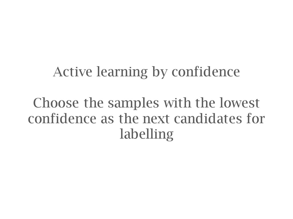
![[Wang14] discusses a few different approaches, confidence being simple and](https://files.speakerdeck.com/presentations/48b8e5fab208446fae0cc8bea631da6a/slide_149.jpg)
![[He15a] He, Zhang, Ren and Sun; Delving Deep into Rectifiers:](https://files.speakerdeck.com/presentations/48b8e5fab208446fae0cc8bea631da6a/slide_175.jpg)
![[He15b] He, Kaiming, et al. "Deep Residual Learning for Image](https://files.speakerdeck.com/presentations/48b8e5fab208446fae0cc8bea631da6a/slide_176.jpg)
![[Hinton12] G.E. Hinton, N. Srivastava, A. Krizhevsky, I. Sutskever and](https://files.speakerdeck.com/presentations/48b8e5fab208446fae0cc8bea631da6a/slide_177.jpg)
![[Ioffe15] Ioffe, S.; Szegedy C.. (2015). “Batch Normalization: Accelerating Deep](https://files.speakerdeck.com/presentations/48b8e5fab208446fae0cc8bea631da6a/slide_178.jpg)
![[Jones87] Jones, J.P.; Palmer, L.A. (1987). "An evaluation of the](https://files.speakerdeck.com/presentations/48b8e5fab208446fae0cc8bea631da6a/slide_179.jpg)
![[Lin13] Lin, Min, Qiang Chen, and Shuicheng Yan. "Network in](https://files.speakerdeck.com/presentations/48b8e5fab208446fae0cc8bea631da6a/slide_180.jpg)
![[Nesterov83] Nesterov, Y. A method of solving a convex programming](https://files.speakerdeck.com/presentations/48b8e5fab208446fae0cc8bea631da6a/slide_181.jpg)
![[Sutskever13] Sutskever, Ilya, et al. On the importance of initialization](https://files.speakerdeck.com/presentations/48b8e5fab208446fae0cc8bea631da6a/slide_182.jpg)
![[Simonyan14] K. Simonyan and Zisserman; Very deep convolutional networks for](https://files.speakerdeck.com/presentations/48b8e5fab208446fae0cc8bea631da6a/slide_183.jpg)
![[Wang14] Wang, Dan, and Yi Shang. "A new active labeling](https://files.speakerdeck.com/presentations/48b8e5fab208446fae0cc8bea631da6a/slide_184.jpg)