Introduction to Hidden Markov Model

A simple introduction to HMM

Transcript

1. An Introduction to HMM Browny 2010.07.21
2. MM vs. HMM States States States Observations
3. Markov Model • Given 3 weather states: – {S1 , S2 , S3 } = {rain, cloudy, sunny} Rain Cloudy Sunny Rain 0.4 0.3 0.3 • What is the probabilities for next 7 days will be {sun, sun, rain, rain, sun, cloud, sun} ? Rain 0.4 0.3 0.3 Cloudy 0.2 0.6 0.2 Sunny 0.1 0.1 0.8
4. Hidden Markov Model • The states –We don’t understand, Hidden! –But it can be indirectly observed • Example –北極or赤道(model), Hot/Cold(state), 1/2/3 ice cream(observation)
5. Hidden Markov Model • The observation is a probability function of state which is not observable directly Hidden States
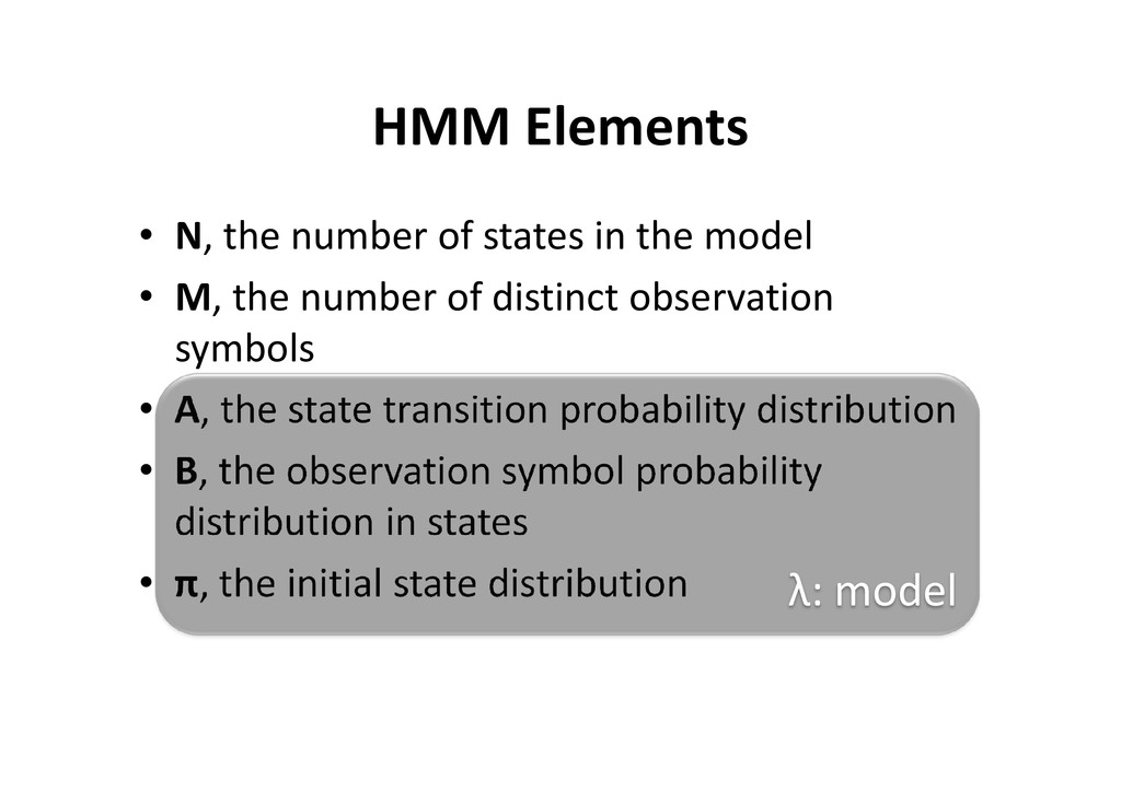
6. HMM Elements • N, the number of states in the model • M, the number of distinct observation symbols • A, the state transition probability distribution • A, the state transition probability distribution • B, the observation symbol probability distribution in states • π, the initial state distribution λ: model
7. Example P(…|C) P(…|H) P(…|Start) P(1|…) 0.7 0.1 P(2|…) 0.2 0.2 B: Observation B: Observation P(3|…) 0.1 0.7 P(C|…) 0.8 0.1 0.5 P(H|…) 0.1 0.8 0.5 P(STOP|…) 0.1 0.1 0 Observation Observation A: Transition A: Transition π: initial π: initial
8. 3 Problems
9. 3 Problems 1. 觀察到的現象最符合哪一個模型 P(觀察到的現象|模型) 2. 怎樣的狀態序列最符合觀察到的現 象和已知的模型 象和已知的模型 P(狀態序列|觀察到的現象, 模型) 3. 怎樣的模型最有可能產生觀察到的 現象 what 模型 maximize P(觀察到的現象| 模型)
10. Solution 1 • 已知模型，一觀察序列之產生機率 P(O|λ) S1 R1 R2 S1 S1 R R1 R2 R R1 R2 R S2 S3 S2 S3 S2 S3 R1 R2 R1 R2 R1 R2 R1 R2 R1 R2 R1 R2 t 1 2 3 觀察到 R1 R1 R2 的機率為多少？
11. Solution 1 • 考慮一特定的狀態序列 • Q = q1 , q2 … qT • 產生出一特定觀察序列之機率為 P(O|Q, λ) = P(O1 |q1 , λ) * P(O2 |q2 , λ) * … * P(Ot |qt , λ) = bq1 (O1 ) * bq2 (O2 ) * … * bqT (OT )
12. Solution 1 • 此一特定序列發生之機率為 • P(O|λ) P(Q|λ) = πq1 * aq1q2 * aq2q3 * … * aq(T-1)qT • 已知模型，一觀察序列之產生機率 P(O|λ) P(O|λ) = P(O|Q, λ) * P(Q| λ) = πq1 * bq1 (O1 ) * aq1q2 bq2 (O2 )* … * aq(T-1)qT * bqT (OT ) 1 2 , ,..., T q q q ∑ 1 2 , ,..., T q q q ∑
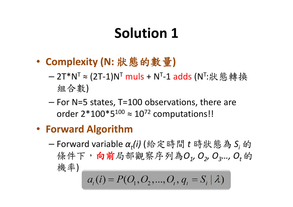
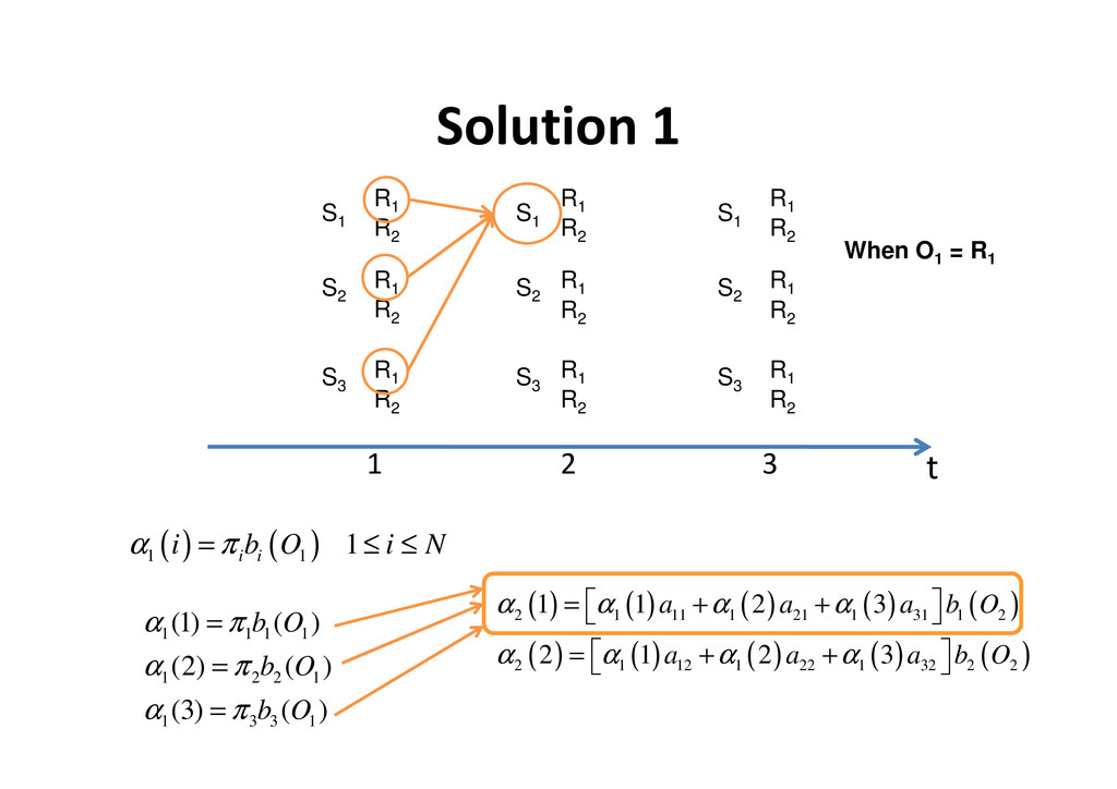
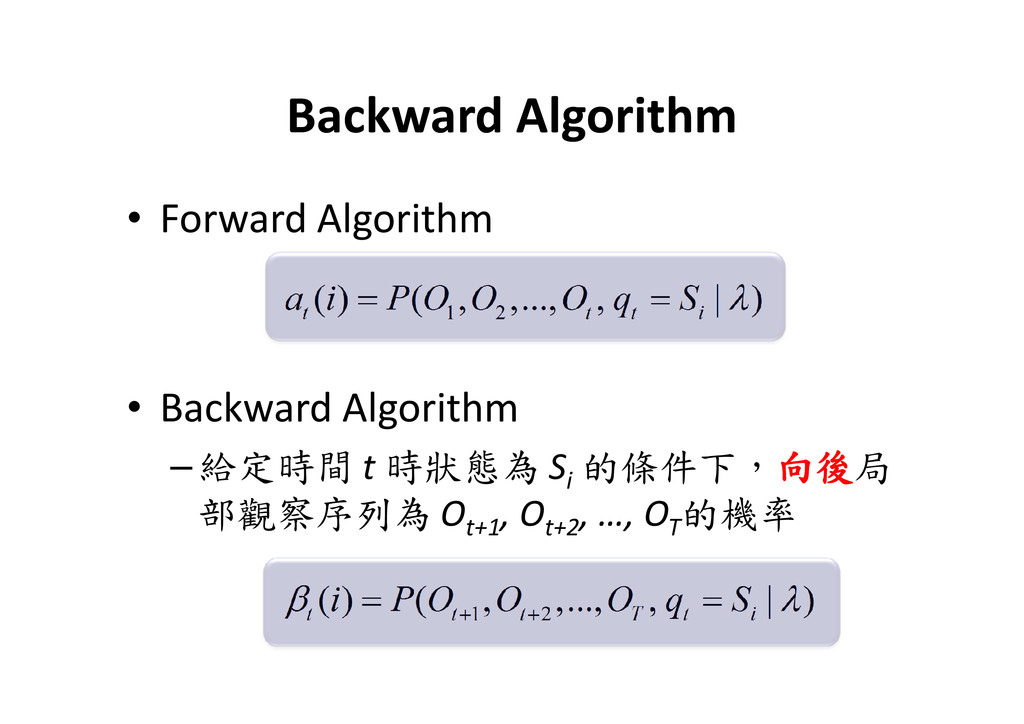
13. Solution 1 • Complexity (N: 狀態的數量 狀態的數量 狀態的數量 狀態的數量) – 2T*NT ≈ (2T-1)NT muls + NT-1 adds (NT:狀態轉換 組合數) – For N=5 states, T=100 observations, there are – For N=5 states, T=100 observations, there are order 2*100*5100 ≈ 1072 computations!! • Forward Algorithm – Forward variable αt (i) (給定時間 t 時狀態為 Si 的 條件下，向前 向前 向前 向前局部觀察序列為O1 , O2 , O3 …, Ot 的 機率) 1 2 ( ) ( , ,..., , | ) t t t i a i P O O O q S λ = =
14. Solution 1 S1 S2 S3 R1 R2 S1 S2 S3 S1 S2 S3 R1 R2 R1 R R1 R2 R1 R2 R1 R R1 R2 R1 R2 R1 R When O1 = R1 R2 R2 R2 1 1 1 1 1 2 2 1 1 3 3 1 (1) ( ) (2) ( ) (3) ( ) b O b O b O α π α π α π = = = ( ) ( ) 1 1 1 i i i b O i N α π = ≤ ≤ ( ) ( ) ( ) ( ) ( ) ( ) ( ) ( ) ( ) ( ) 2 1 11 1 21 1 31 1 2 2 1 12 1 22 1 32 2 2 1 1 2 3 2 1 2 3 a a a b O a a a b O α α α α α α α α = + +     = + +     t 1 2 3
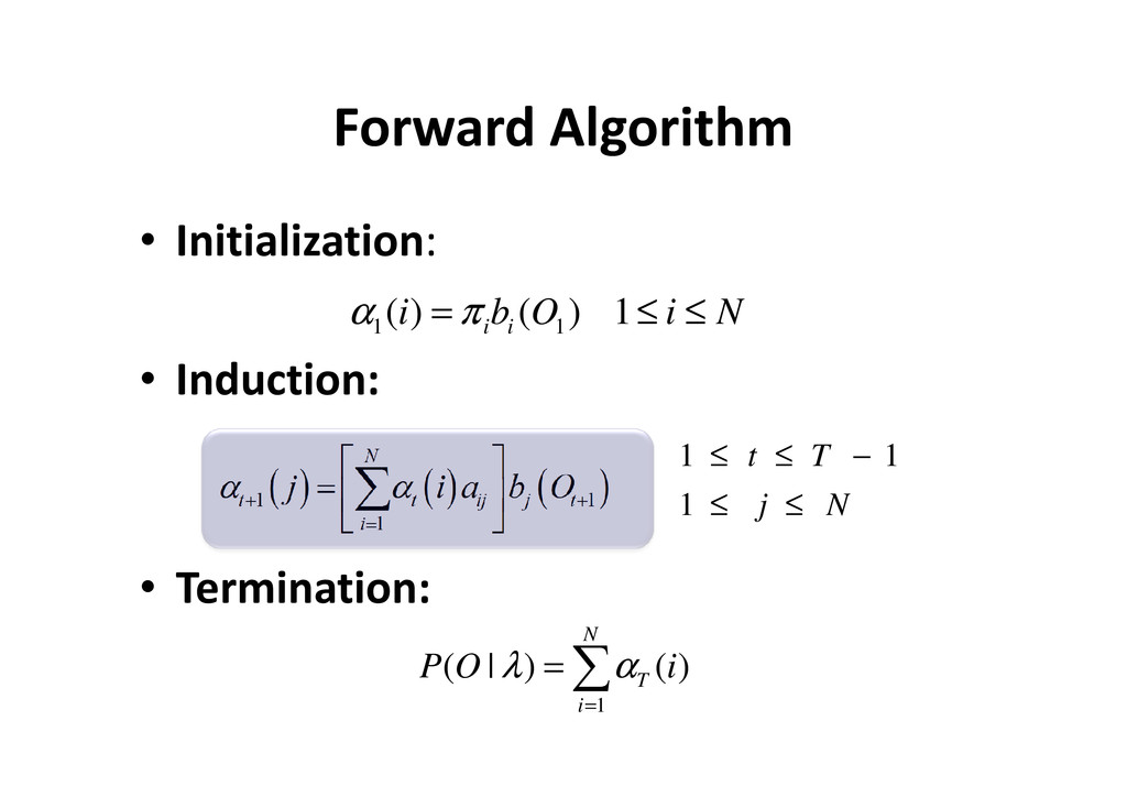
15. Forward Algorithm • Initialization: • Induction: 1 1 ( ) ( ) 1 i i i b O i N α π = ≤ ≤ • Induction: • Termination: ( ) ( ) ( ) 1 1 1 N t t ij j t i j i a b O α α + + =   =     ∑ 1 1 1 t T j N ≤ ≤ − ≤ ≤ 1 ( | ) ( ) N T i P O i λ α = = ∑
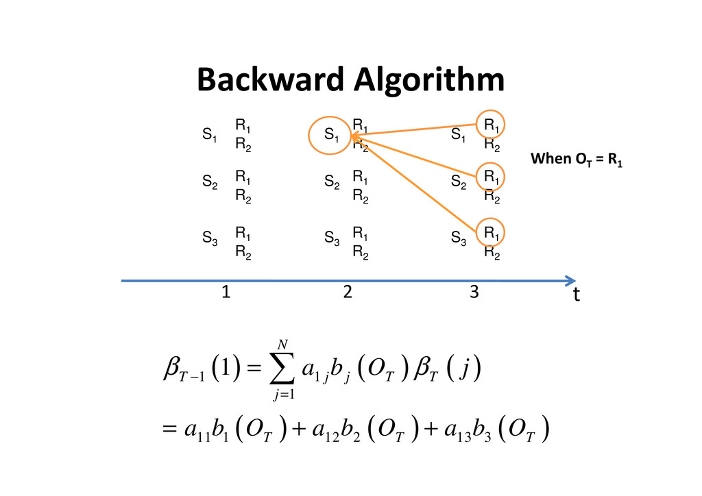
16. Backward Algorithm • Forward Algorithm 1 2 ( ) ( , ,..., , | ) t t t i a i P O O O q S λ = = • Backward Algorithm –給定時間 t 時狀態為 Si 的條件下，向後 向後 向後 向後局 部觀察序列為 Ot+1 , Ot+2 , …, OT 的機率 1 2 ( ) ( , ,..., , | ) t t t T t i i P O O O q S β λ + + = =
17. Backward Algorithm • Initialization • Induction ( ) 1 1 T i i N β = ≤ ≤ • Induction 1 1 1 ( ) ( ) ( ) N t ij j t t j i a b O j β β + + = = ∑ 1, 2,...,1 1 t T T i N = − − ≤ ≤
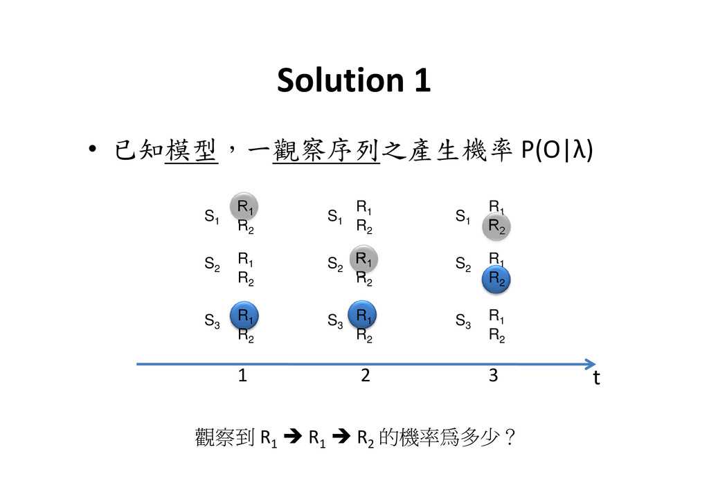
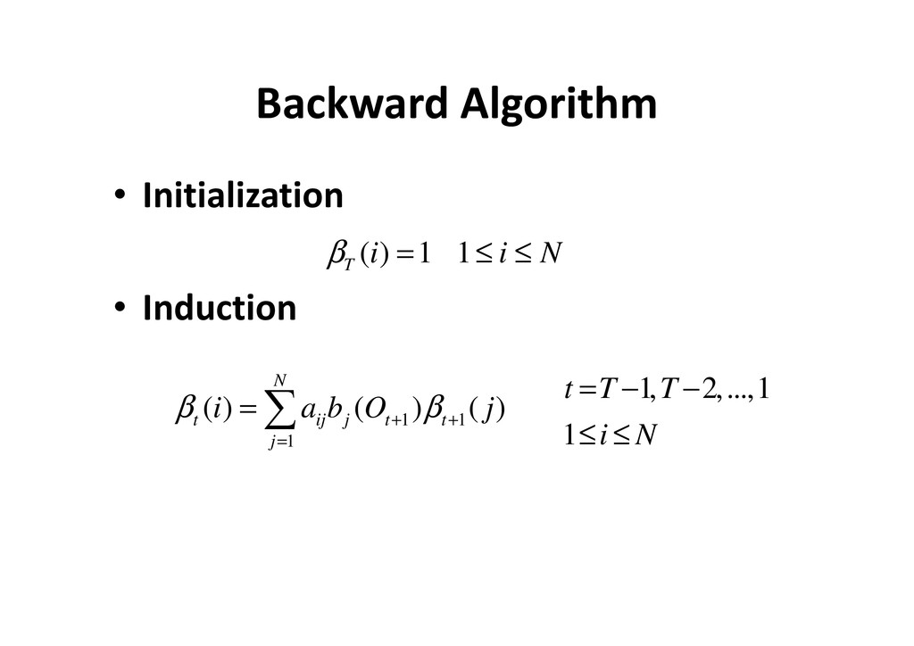
18. Backward Algorithm S1 S2 S3 R1 R2 S1 S2 S3 S1 S2 S3 R1 R2 R1 R R1 R2 R1 R2 R1 R R1 R2 R1 R2 R1 R When OT = R1 R2 R2 R2 ( ) ( ) ( ) ( ) ( ) ( ) 1 1 1 11 1 12 2 13 3 1 N T j j T T j T T T a b O j a b O a b O a b O β β − = = = + + ∑ t 1 2 3
19. Solution 2 • 怎樣的狀態序列最能解釋觀察到的現 象和已知的模型 P(狀態序列|觀察到的現象, 模型) • 無精確解，有很多種方式解此問題， 對狀態序列的不同限制 對狀態序列的不同限制 對狀態序列的不同限制 對狀態序列的不同限制有不同的解法
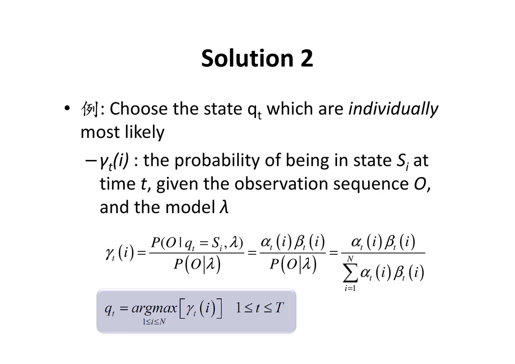
20. Solution 2 • 例: Choose the state qt which are individually most likely –γt (i) : the probability of being in state Si at time t, given the observation sequence O, time t, given the observation sequence O, and the model λ ( ) ( ) ( ) ( ) ( ) ( ) ( ) ( ) ( ) ( ) 1 1 ( | , ) 1 t t t t t i t N t t i t t i N i i i i P O q S i P O P O i i q argmax i t T α β α β λ γ λ λ α β γ = ≤ ≤ = = = = = ≤ ≤     ∑
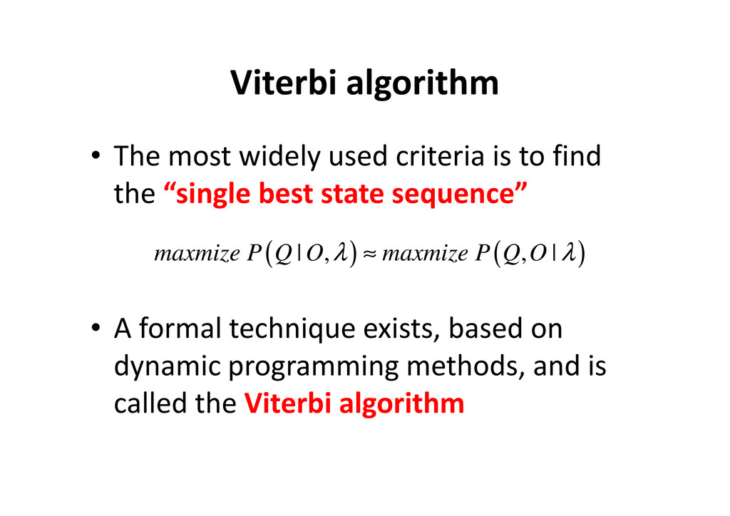
21. Viterbi algorithm • The most widely used criteria is to find the “single best state sequence” ( ) ( ) | , , | maxmize P Q O maxmize P Q O λ λ ≈ • A formal technique exists, based on dynamic programming methods, and is called the Viterbi algorithm ( ) ( ) | , , | maxmize P Q O maxmize P Q O λ λ ≈
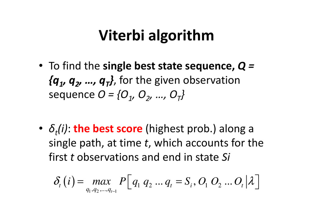
22. Viterbi algorithm • To find the single best state sequence, Q = {q1 , q2 , …, qT }, for the given observation sequence O = {O1 , O2 , …, OT } • δt (i): the best score (highest prob.) along a single path, at time t, which accounts for the first t observations and end in state Si ( ) 1 2 1 1 2 1 2 , ,..., ... , ... t t t i t q q q i max P q q q S O O O δ λ − =  =   
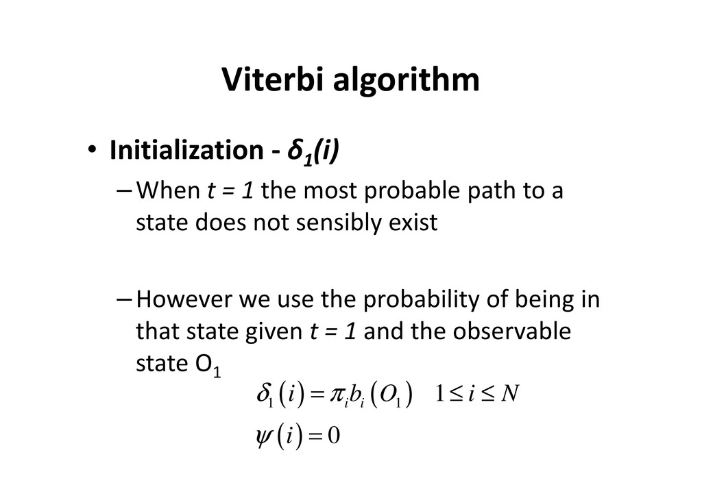
23. Viterbi algorithm • Initialization - δ1 (i) –When t = 1 the most probable path to a state does not sensibly exist –However we use the probability of being in that state given t = 1 and the observable state O1 ( ) ( ) ( ) 1 1 1 0 i i i b O i N i δ π ψ = ≤ ≤ =
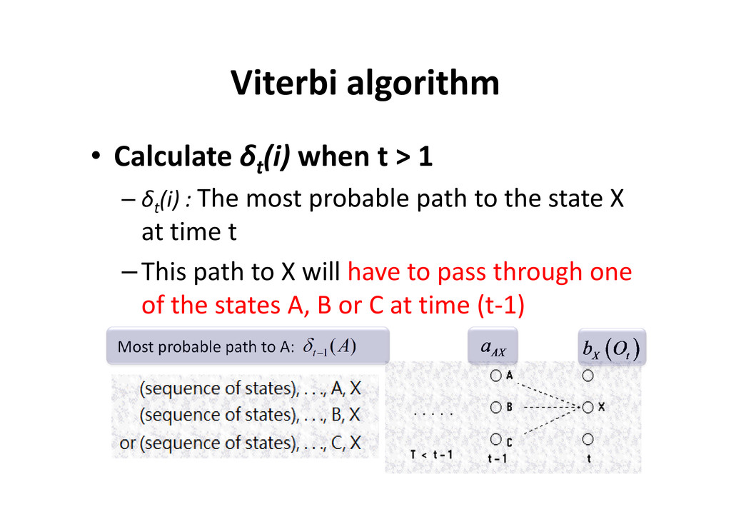
24. Viterbi algorithm • Calculate δt (i) when t > 1 – δt (i) : The most probable path to the state X at time t –This path to X will have to pass through one –This path to X will have to pass through one of the states A, B or C at time (t-1) Most probable path to A: 1 ( ) t A δ − AX a ( ) X t b O
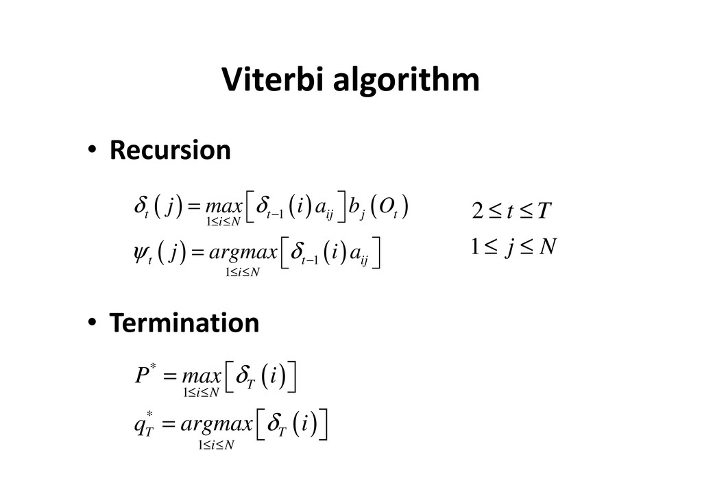
25. Viterbi algorithm • Recursion ( ) ( ) ( ) ( ) ( ) 1 1 t t ij j t i N j max i a b O j argmax i a δ δ ψ δ − ≤ ≤   =     =   2 1 t T j N ≤ ≤ ≤ ≤ • Termination ( ) ( ) 1 1 t t ij i N j argmax i a ψ δ − ≤ ≤   =   1 j N ≤ ≤ ( ) ( ) * 1 * 1 T i N T T i N P max i q argmax i δ δ ≤ ≤ ≤ ≤ =     =    
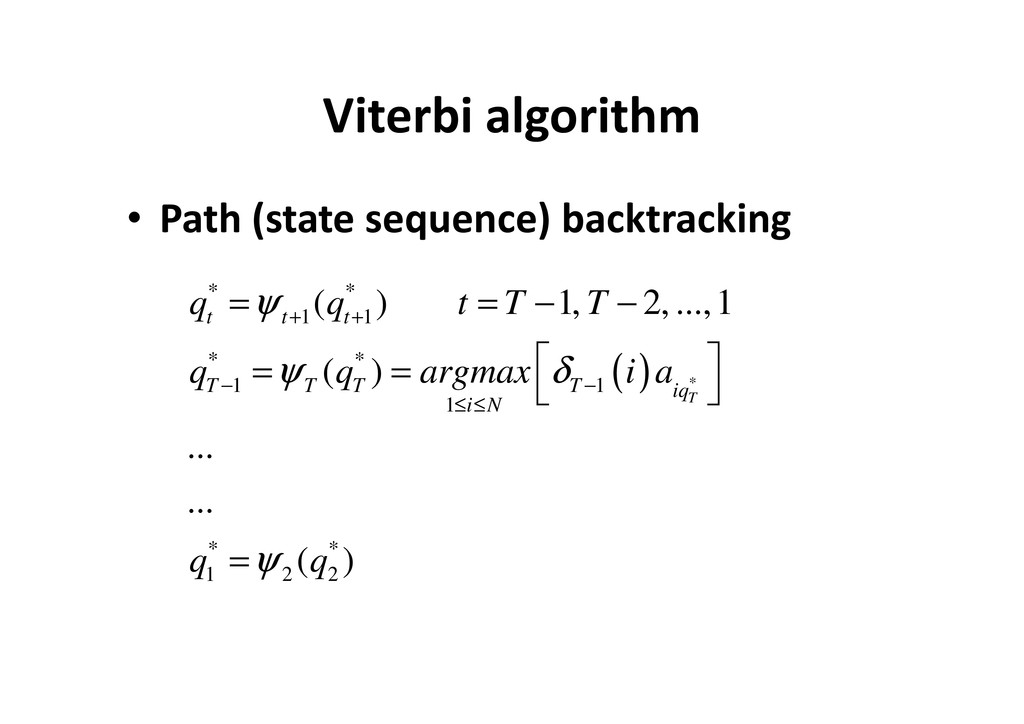
26. Viterbi algorithm • Path (state sequence) backtracking ( ) * * 1 1 * * ( ) 1, 2, ...,1 ( ) t t t q q t T T q q argmax i a ψ ψ δ + + = = − −   = = ( ) * * * 1 1 1 * * 1 2 2 ( ) ... ... ( ) T T T T T iq i N q q argmax i a q q ψ δ ψ − − ≤ ≤   = =   =
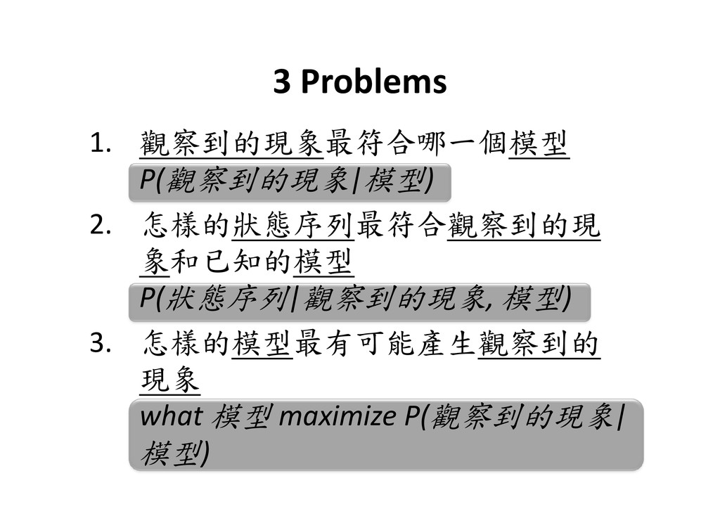
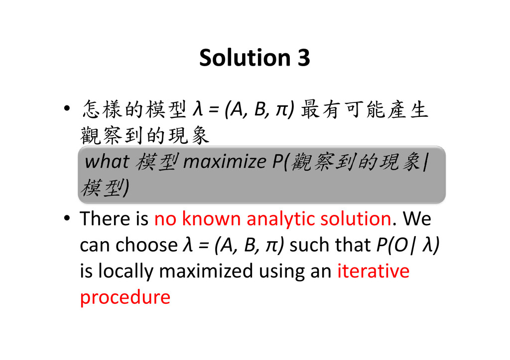
27. Solution 3 • 怎樣的模型 λ = (A, B, π) 最有可能產生 觀察到的現象 what 模型 maximize P(觀察到的現象| 模型) 模型) • There is no known analytic solution. We can choose λ = (A, B, π) such that P(O| λ) is locally maximized using an iterative procedure
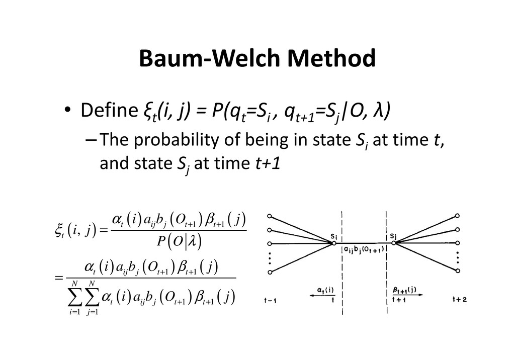
28. Baum-Welch Method • Define ξt (i, j) = P(qt =Si , qt+1 =Sj |O, λ) –The probability of being in state Si at time t, and state Sj at time t+1 ( ) ( ) ( ) ( ) ( ) ( ) ( ) ( ) ( ) ( ) ( ) 1 1 1 1 1 1 1 1 , t ij j t t t t ij j t t N N t ij j t t i j i a b O j i j P O i a b O j i a b O j α β ξ λ α β α β + + + + + + = = = = ∑∑
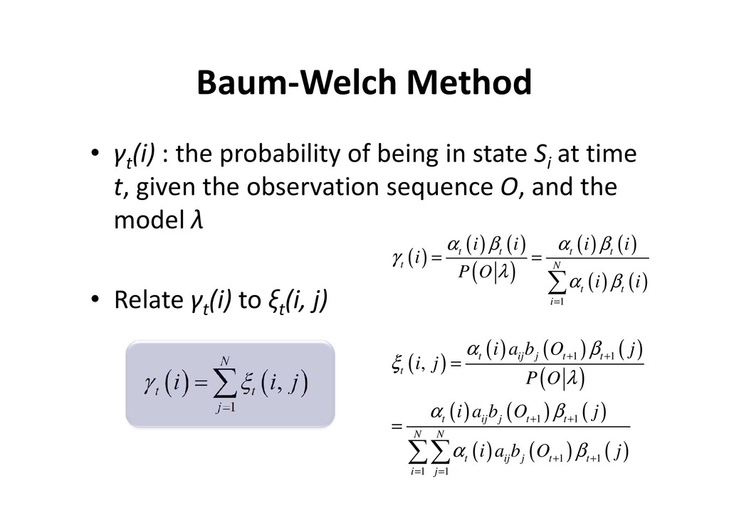
29. Baum-Welch Method • γt (i) : the probability of being in state Si at time t, given the observation sequence O, and the model λ ( ) ( ) ( ) ( ) ( ) ( ) t t t t i i i i i α β α β γ = = • Relate γt (i) to ξt (i, j) ( ) ( ) ( ) ( ) 1 t N t t i i P O i i γ λ α β = = = ∑ ( ) ( ) ( ) ( ) ( ) ( ) ( ) ( ) ( ) ( ) ( ) 1 1 1 1 1 1 1 1 , t ij j t t t t ij j t t N N t ij j t t i j i a b O j i j P O i a b O j i a b O j α β ξ λ α β α β + + + + + + = = = = ∑∑ ( ) ( ) 1 , N t t j i i j γ ξ = = ∑
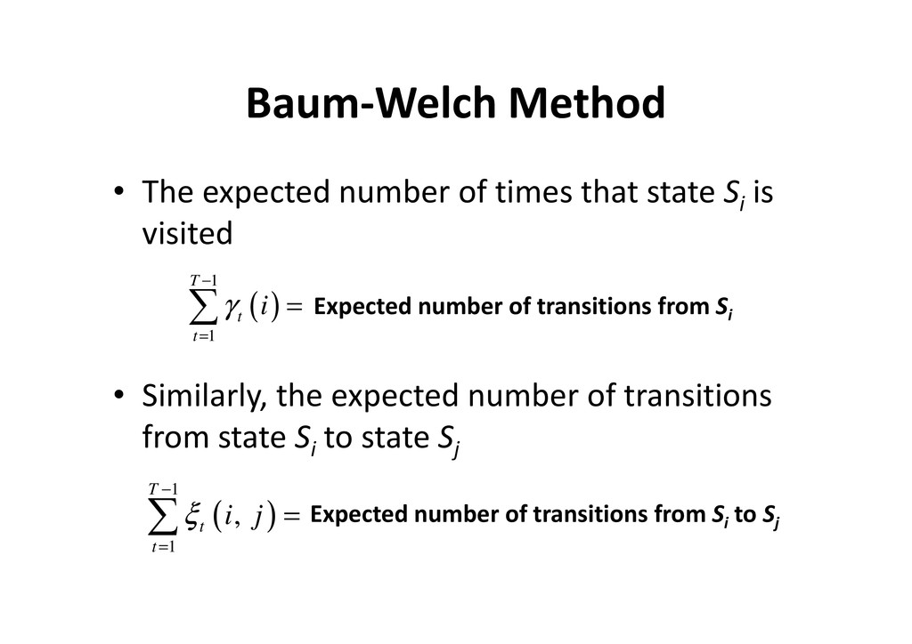
30. Baum-Welch Method • The expected number of times that state Si is visited ( ) 1 T t i γ − = ∑ Expected number of transitions from Si • Similarly, the expected number of transitions from state Si to state Sj ( ) 1 t t= ∑ ( ) 1 1 , T t t i j ξ − = = ∑ Expected number of transitions from Si to Sj
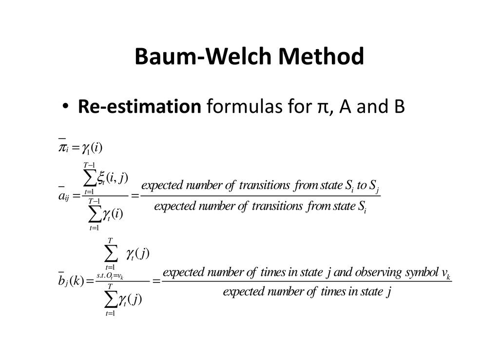
31. Baum-Welch Method • Re-estimation formulas for π, A and B 1 1 ( ) ( , ) i T i i j π γ ξ − = ∑ 1 1 1 1 . . 1 ( , ) ( ) ( ) ( ) ( ) t k t i j t ij T i t t T t t s t O v j T t t i j expected number of transitions fromstate S toS a expected number of transitions fromstate S i j expected number of timesinstate j and observing symb b k j ξ γ γ γ = − = = = = = = = = ∑ ∑ ∑ ∑ k ol v expected number of timesinstate j
32. Baum-Welch Method • P(O|λ) > P(O|λ) • Iteratively use λ in place of λ and repeat • Iteratively use λ in place of λ and repeat the re-estimation, we then can improve P(O| λ) until some limiting point is reached