Institute of Technology [Music Mind and Machine] Daniel P.W. Ellis Assistant Professor of Electrical Engineering Columbia University [LabROSA] Deb Roy Associate Professor of Media Arts & Sciences Massachusetts Institute of Technology [Cognitive Machines]
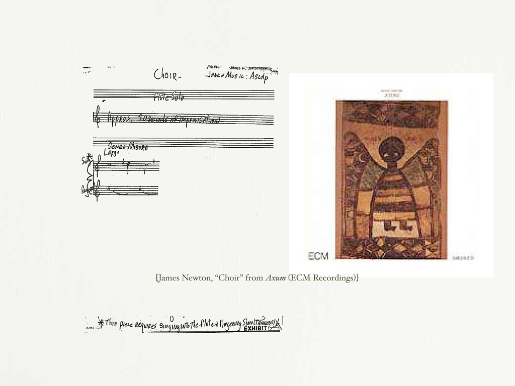
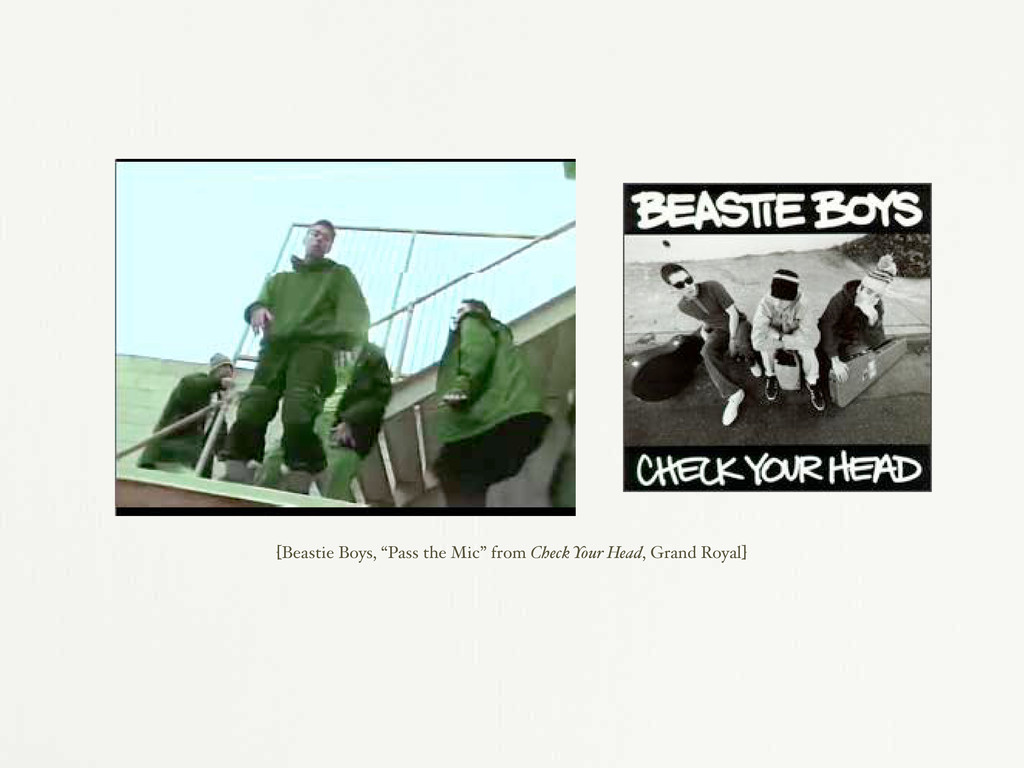
8 9 10 11 12 13 14 15 16 17 18 19 20 21 22 23 24 25 JEFFREY A. BERCHENKO, SBN 094902 LAW OFFICE OF JEFFREY BERCHENKO 240 Stockton Street, 3rd Floor San Francisco, California 94108 (415) 362-5700; Fax (415) 362-4119 Attorneys for Plaintiff James W. Newton, Jr. dba Janew Music UNITED STATES DISTRICT COURT CENTRAL DISTRICT OF CALIFORNIA JAMES W. NEWTON, JR. dba ) JANEW MUSIC, ) Case No. CV 00-04909-NM (MANx) ) Plaintiff, ) FIRST AMENDED COMPLAINT ) (COPYRIGHT INFRINGEMENT -- v. ) 17 U.S.C. §101 et seq.) ) MICHAEL DIAMOND, ADAM HOROVITZ ) and ADAM YAUCH, dba BEASTIE BOYS,) a New York Partnership, CAPITOL ) DEMAND FOR JURY TRIAL RECORDS, INC., a Delaware ) Corporation, GRAND ROYAL RECORDS,) INC., a California Corporation, ) UNIVERSAL POLYGRAM INTERNATIONAL) PUBLISHING, INC., a Delaware ) Corporation, BROOKLYN DUST MUSIC,) an entity of unknown origin, ) MARIO CALDATO, JR., an ) individual, JANUS FILMS, LLC, a ) New York Limited Liability ) Company, CRITERION COLLECTION, a ) California Partnership, VOYAGER ) PUBLISHING COMPANY, INC., a ) Delaware Corporation, SONY MUSIC) ENTERTAINMENT, INC.,A Delaware ) Corporation, BMG DIRECT )
300 Jan 11 Jan 12 Jan 13 Jan 14 Jan 15 Jan 16 Jan 17 Jan 18 Jan 19 Jan 20 Jan 21 Jan 22 Jan 23 Jan 24 Jan 25 Jan 26 Jan 27 Jan 28 Jan 29 Jan 30 Jan 31 Feb 1 Feb 2 Feb 3 Feb 4 Feb 5 Feb 6 Feb 7 Feb 8 Feb 9 Feb 10 Feb 11 Feb 12 Feb 13 Feb 14 Feb 15 Feb 16 Feb 17 Feb 18 Feb 19 Feb 20 Feb 21 Feb 22 Feb 23 Feb 24 Feb 25 Feb 26 Feb 27 Feb 28 Mar 1 Mar 2 Mar 3 Mar 4 Mar 5 Mar 6 Mar 7 Mar 8 Mar 9 Mar 10 Mar 11 Mar 12 Mar 13 Mar 14 Mar 15 Mar 16 Mar 17 Mar 18 Mar 19 Mar 20 Mar 21 Mar 22 Mar 23 Mar 24 Mar 25 Mar 26 Mar 27 Mar 28 Mar 29 Mar 30 Mar 31 Apr 1 Apr 2 Apr 3 Apr 4 Apr 5 Apr 6 Apr 7 Apr 8 Apr 9 73 41 49 21 2 26 3 119 140 13 48 13 13 1 93 3 9 21 169 2 1 43 14 3 21 20 14 22 64 31 261 237 14 5 21 37 96 17 37 29 87 225 16 4 3 1 1 1 2 3
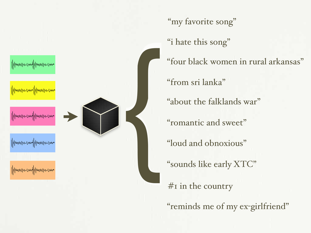
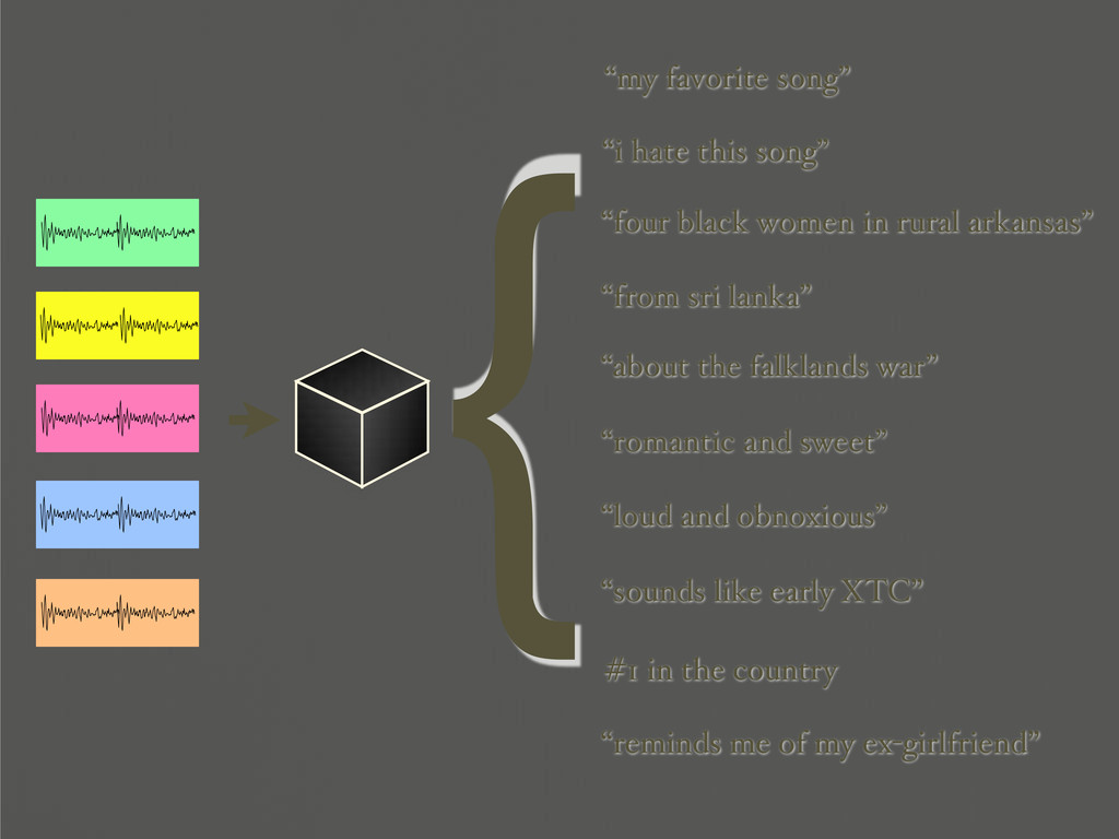
in rural arkansas” “from sri lanka” “about the falklands war” “romantic and sweet” “loud and obnoxious” “sounds like early XTC” #1 in the country “reminds me of my ex-girlfriend” {
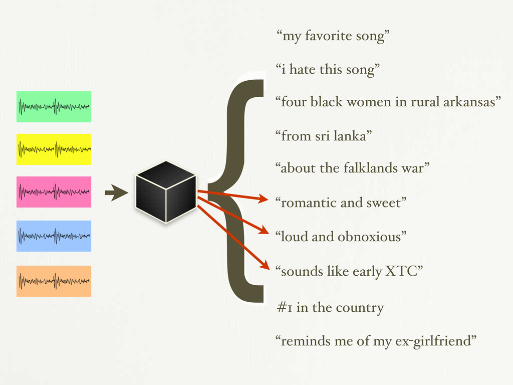
in rural arkansas” “from sri lanka” “about the falklands war” “romantic and sweet” “loud and obnoxious” “sounds like early XTC” #1 in the country “reminds me of my ex-girlfriend” {
in rural arkansas” “from sri lanka” “about the falklands war” “romantic and sweet” “loud and obnoxious” “sounds like early XTC” #1 in the country “reminds me of my ex-girlfriend” {
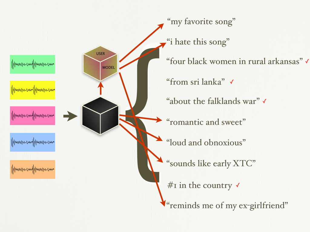
in rural arkansas” “from sri lanka” “about the falklands war” “romantic and sweet” “loud and obnoxious” “sounds like early XTC” #1 in the country “reminds me of my ex-girlfriend” { MODEL USER
in rural arkansas” “from sri lanka” “about the falklands war” “romantic and sweet” “loud and obnoxious” “sounds like early XTC” #1 in the country “reminds me of my ex-girlfriend” { MODEL USER ✓ ✓ ✓ ✓
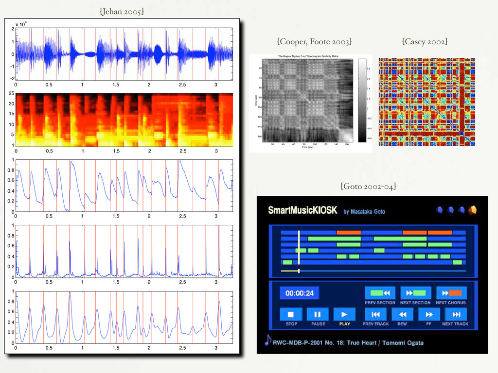
and Acoustics October 19-22, 2003, New Paltz, NY mented training data. In contrast, our technique uses the digital audio to model itself for both segmentation and clustering. Tzane- takis and Cook [6] discuss “audio thumbnailing” using a segmen- tation based method in which short segments near segmentation boundaries are concatenated. This is similar to “time-based com- pression” of speech [7]. In contrast, we use complete segments for summaries, and we do not alter playback speed. Previous work by the authors has also used similarity matrices for excerpting, with- out an explicit segmentation step [8]. The present method results in a structural characterization, and is far more likely to start or end the summary excerpts on actual segment boundaries. We have also presented an earlier version of this approach, however with less complete validation [4]. 2.2. Media Segmentation, Clustering, & Similarity Analysis Our clustering approach is inspired by methods developed for seg- menting still images [9]. Using color, texture, or spatial sim- ilarity measures, a similarity matrix is computed between pixel pairs. This similarity matrix is then factorized into eigenvectors and eigenvalues. Ideally, the foreground and background pixels ex- hibit within-class similarity and between-class dissimilarity. Thus thresholding the eigenvector corresponding to the largest eigen- value can classify the pixels into foreground and background. In contrast, we employ a related technique to cluster time-ordered data. Gong and Liu have presented an SVD based method for video summarization [10], by factorizing a rectangular time-feature matrix, rather than a square similarity matrix. Cutler and Davis use affinity matrices to analyze periodic motion using a correlation- based method [11]. 3. SIMILARITY ANALYSIS 3.1. Constructing the similarity matrix Similarity analysis is a non-parametric technique for studying the global structure of time-ordered streams. First, we calculate 80-bin spectrograms from the short time Fourier transform (STFT) of 0.05 second non-overlapping frames in the source audio. Each frame is Hamming-windowed, and the logarithm of the magnitude of the FFT is binned into an 80-dimensional vector. We have also ex- !0.6 !0.4 !0.2 0 0.2 0.4 0.6 0.8 Time (sec) Time (sec) "The Magical Mystery Tour" Spectrogram Similarity Matrix 20 40 60 80 100 120 140 160 20 40 60 80 100 120 140 160 0 20 40 60 80 100 120 140 160 180 0 0.1 0.2 0.3 0.4 0.5 0.6 0.7 0.8 0.9 1 Time (seconds) Novelty Score: The Magical Mystery Tour Figure 2: Top: The similarity matrix computed from the song “The Magical Mystery Tour ” by The Beatles. Bottom: the time- indexed novelty score produced by correlating the checkerboard kernel along the main diagonal of the similarity matrix. squares along the main diagonal. Brighter rectangular regions off the main diagonal indicate similarity between segments. 3.2. Audio Segmentation [Cooper, Foote 2003] [Casey 2002] [Goto 2002-04] “Unsemantic” music-IR (what works) 0 0.5 1 1.5 2 2.5 3 ! -2 ! -1 0 1 2 x 10⁴ 0 0.5 1 1.5 2 2.5 3 0 0.2 0.4 0.6 0.8 1 0 0.2 0.4 0.6 0.8 1 0 0.2 0.4 0.6 0.8 1 1 5 10 15 20 25 0 0.5 1 1.5 2 2.5 3 0 0.5 1 1.5 2 2.5 3 0 0.5 1 1.5 2 2.5 3 [Jehan 2005]
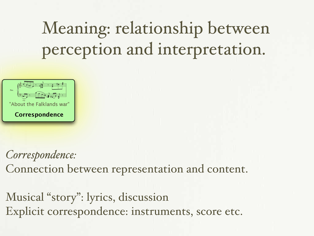
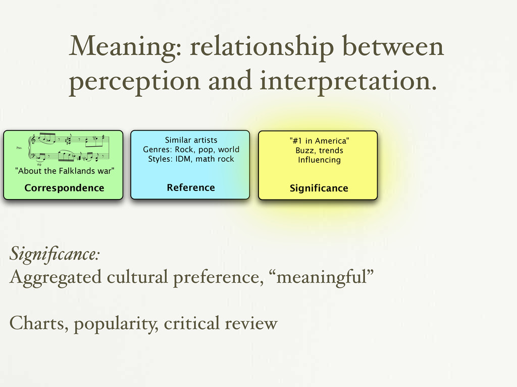
œ b œ ‰ œ œ œ . # # # j ‰ œ œ . œ . <n> œ œ . ? mp œ b œ ‰ œ œ œ œ b œ œ œ b j œ <n> œ œ œ j ‰ "About the Falklands war" Reference Similar artists Genres: Rock, pop, world Styles: IDM, math rock Reference: Connection between music and other music. Similar artists, styles, genres
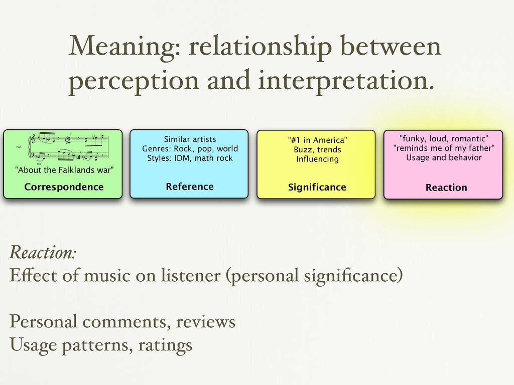
œ b œ ‰ œ œ œ . # # # j ‰ œ œ . œ . <n> œ œ . ? mp œ b œ ‰ œ œ œ œ b œ œ œ b j œ <n> œ œ œ j ‰ "About the Falklands war" Reference Similar artists Genres: Rock, pop, world Styles: IDM, math rock Significance "#1 in America" Buzz, trends Influencing Reaction "funky, loud, romantic" "reminds me of my father" Usage and behavior Reaction: Effect of music on listener (personal significance) Personal comments, reviews Usage patterns, ratings
grass tiger jet plane sky We build a system that has these functions, called SAR (semantic–audio retrieval), by learning the connection between a semantic space and an auditory space. Semantic space maps words into a high-dimensional probabilistic space. Acoustic space describes sounds by a multidimensional vector. In general, the connection between these two spaces will be many to many. Horse sounds, for example, might include footsteps and neighs. Figure 1 shows one half of SAR; how to retrieve sounds from words. Annotations that describe sounds are clustered within a hierarchical semantic model that uses multinomial models. The sound files, or acoustic documents, that correspond to each node in the semantic hierarchy are modeled with Gaussian mixture models (GMMs). Given a semantic request, SAR identifies the portion of the semantic space that best fits the request, and then measures the likelihood that each sound in the database fits the 2. THE EXISTING SYSTEMS There are many multimedia retrieval systems that use a comb tion of words and/or examples to retrieve audio (and video) users. An effective way to find an image of the space shuttle i enter the words “space shuttle jpg” into a text-based web sea engine. The original Google system did not know about ima but, fortunately, many people created web pages with the ph “space shuttle” that contained a JPEG image of the shuttle. M recently, both Google and AltaVista for images, and Compus ics for audio, have built systems that automate these searc They allow people to look for images and sound based on nea words. The SAR work expands those search techniques by c sidering the acoustic and semantic similarity of sounds to al Semantic Space Acoustic Space Step Whinny Figure 1: SAR models all of semantic space with a hierarchical collection of multinomial models, each portion in the semantic model is linked to equivalent sound documents in acoustic space with a GMM. Semantic Space Acoustic Space Horse Trot Figure 2: SAR describes with words an audio query by partit ing the audio space with a set of hierarchical acoustic models then linking each set of audio files (or documents) to a proba ity model in semantic space. rate tracks, with 330 minutes of audio recordings of animal sounds. In addition, the concatenated name of the CD (e.g., “Horses I”) and track description (e.g., “One horse eating hay and moving around”) form a unique semantic label for each track. The audio from the CD track and the liner notes form a pair of acoustic and semantic documents used to train the SAR system. 2. THE EXISTING SYSTEMS There are many multimedia retrieval systems that use a combina- tion of words and/or examples to retrieve audio (and video) for users. An effective way to find an image of the space shuttle is to enter the words “space shuttle jpg” into a text-based web search engine. The original Google system did not know about images, but, fortunately, many people created web pages with the phrase “space shuttle” that contained a JPEG image of the shuttle. More recently, both Google and AltaVista for images, and Compuson- ics for audio, have built systems that automate these searches. They allow people to look for images and sound based on nearby words. The SAR work expands those search techniques by con- sidering the acoustic and semantic similarity of sounds to allow Semantic Space Acoustic Space Horse Trot Figure 2: SAR describes with words an audio query by partition- ing the audio space with a set of hierarchical acoustic models and then linking each set of audio files (or documents) to a probabil- ity model in semantic space. [Slaney 2002] [Roy, Hsiao, Mavridis, Gorniak 2001-05] Grounding
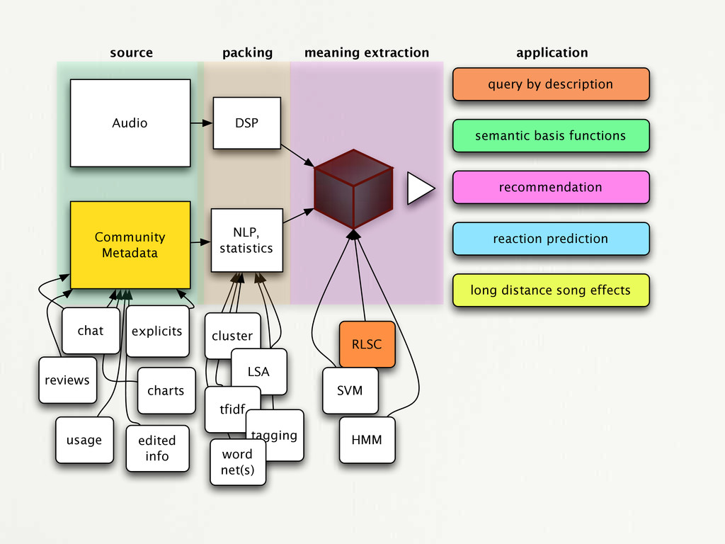
edited info explicits query by description semantic basis functions recommendation reaction prediction long distance song effects source packing meaning extraction application cluster LSA tfidf tagging word net(s) RLSC SVM HMM
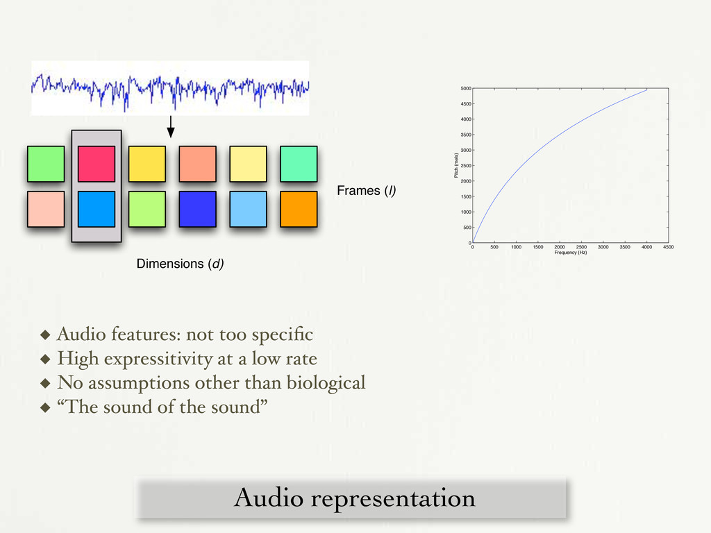
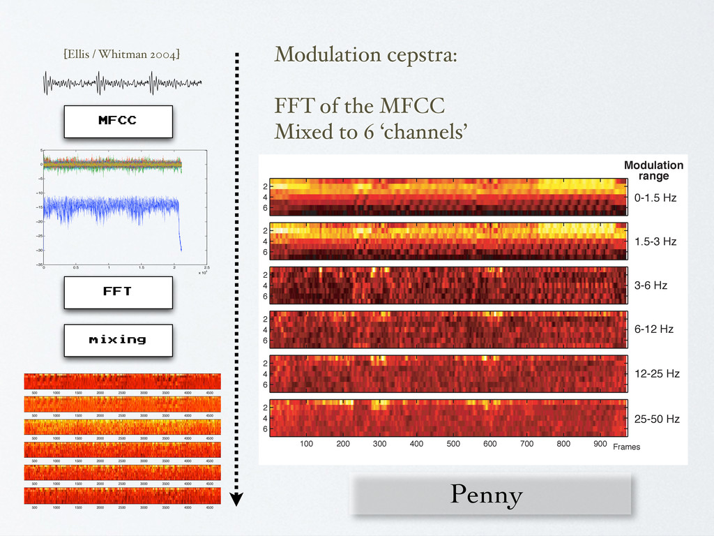
0 500 1000 1500 2000 2500 3000 3500 4000 4500 5000 Frequency (Hz) Pitch (mels) Figure 3-7: Mel scale: mels vs. frequency in Hz. ! "! #! !%" !%! !& !$ !# !" ! '()*+, ! "! #! $! !!-" ! !-" !-# !-$ !-& % %-" '()*+, ! "! #! $! !% !!-& !!-$ !!-# !!-" ! !-" !-# !-$ '()*+, Figure 3-8: Penny V1, 2 and 3 for the first 60 seconds of “Shipbuilding.” To compute modulation cepstra we start with MFCCs at a cepstral frame rate (o between 5 Hz and 100 Hz), returning a vector of 13 bins per audio frame. We then s successive time samples for each MFCC bin into 64 point vectors and take a sec Fourier transform on these per-dimension temporal energy envelopes. We aggre Audio representation Frames (l) Dimensions (d) ◆ Audio features: not too specific ◆ High expressitivity at a low rate ◆ No assumptions other than biological ◆ “The sound of the sound”
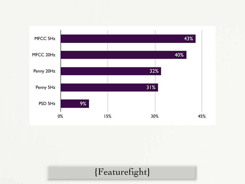
5Hz 0% 15% 30% 45% Figure 3-10: Evaluation of five features in a 1-in-20 artist ID task. is still a valuable feature for us: low data rate and time representation. Because of the overlap in the fourier analysis of the cepstral frames, the Penny data rate is a fraction of the cepstral rate. In usual implementation (Penny with a cepstral frame rate of 5 Hz, 300 MFCC frames per minute) we end up with 45 Penny frames per minute of audio. Even if MFCCs outperform at equal cepstral analysis rates, Penny needs far less actual
in the representer theorem, where a high d x can be represented fully by a generalized dot product (in a Re t Space [7]) between x i and x j using a kernel function K(x binary classification problem shown in figure 5-1 could be clas hyperplane learned by an SVM. However, non-linearly sepa -2 need to consider a new topology, and we can substitute in n that represents data as Kf (x1, x2 ) = e (|x1 x2|)2 2 nable parameter. Kernel functions can be viewed as a ‘distanc all the high-dimensionality points in your input feature spac 0.3 0.32 0.34 0.36 0.38 0.4 0.42 0.44 0.46 3 3.5 4 4.5 5 5.5 6 rock dance rap 50 100 150 200 20 40 60 80 100 120 140 160 180 200
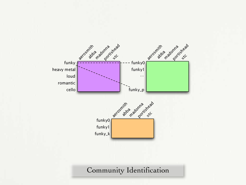
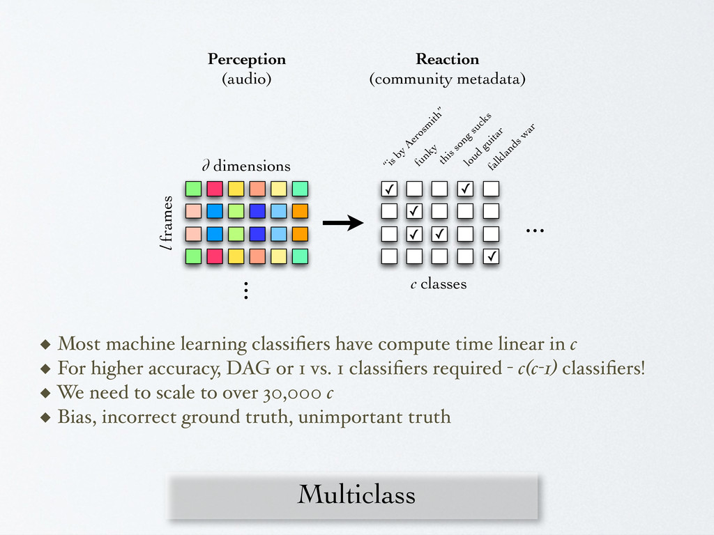
this song sucks loud guitar falklands w ar ✓ ✓ ✓ ✓ ✓ ✓ ... ... c classes ◆ Most machine learning classifiers have compute time linear in c ◆ For higher accuracy, DAG or 1 vs. 1 classifiers required - c(c-1) classifiers! ◆ We need to scale to over 30,000 c ◆ Bias, incorrect ground truth, unimportant truth Perception (audio) Reaction (community metadata)
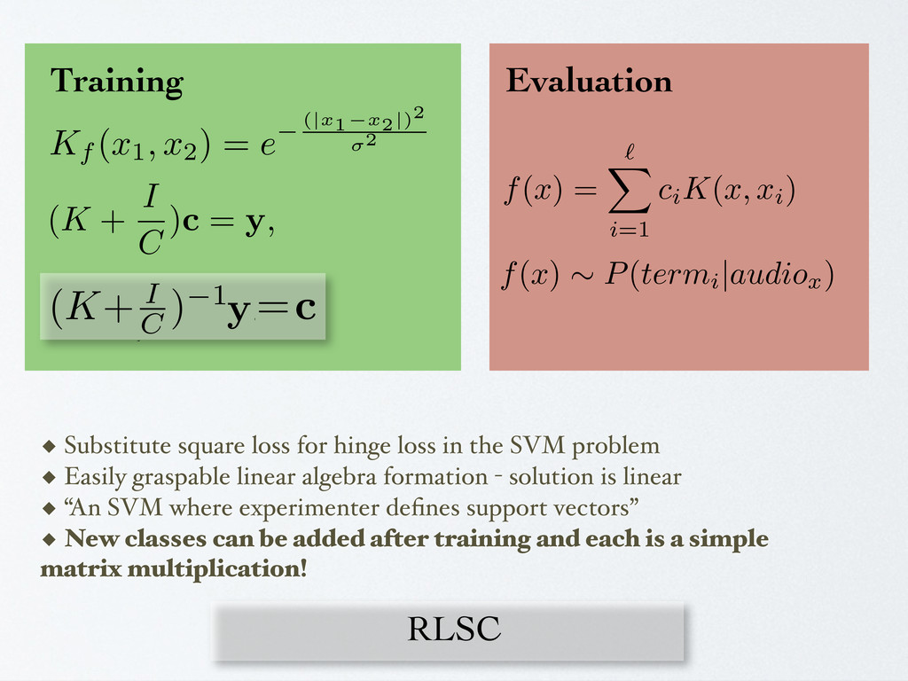
SVM problem ◆ Easily graspable linear algebra formation - solution is linear ◆ “An SVM where experimenter defines support vectors” ◆ New classes can be added after training and each is a simple matrix multiplication! RLSC system consists of solving the sys- uations (K + I C )c = y, (2) ernel matrix, c is a classifier ‘machine,’ y , and C is a user-supplied regularization we keep at 10. 1 The crucial property of ask is that if we store the inverse matrix n for a new right-hand side y (i.e. a new values we are trying to predict), we can w classifier c via a simple matrix multipli- SC is very well-suited to problems of this d set of training observations and a large lowest two modulati ture across all cepstr use a 10 Hz feature f 1 Hz. We split the a half of the albums in scribed above we com data and then invert, review corpus. 7.2. Evaluation of To evaluate the mod testing gram matrix a f (x1, x2 ) = e (|x1 x2|) 2 (1) meter we keep at 0.5. an RLSC system consists of solving the equations (K + I C ) c = y , (2) r-supplied regularization constant. The ued classification function f is f(x) = X i=1 ciK(x, xi ). (3) P(an ) in fined as even in th Now w threshold P(at ) gr manner w scoring c or unimp 6 Lin Disc real-valued classification function f is f(x) = X i=1 ciK(x, xi ). (3) al property of RLSC is that if we store the in- rix (K+ I C ) 1, then for a new right-hand side y , ompute the new c via a simple matrix multipli- his allows us to compute new classifiers (after the data and storing it in memory) on the fly ple matrix multiplications. aluation for a “Query-by-Description” Task ate our connection-finding system, we compute or un 6 L D Give our m terms mode senso ing a hear terms datio on f is (3) we store the in- ght-hand side y , matrix multipli- classifiers (after mory) on the fly cription” Task em, we compute or unimportant. 6 Linguistic Experts for Pa Discovery Given a set of ‘grounded’ single ter our method for uncovering paramete terms and learning the knobs to vary model states that certain knowledge sensory input or intrinsic knowledge ing a ‘linguistic expert.’ If we hear hear ‘quiet’ audio, we would need terms are antonymially related befo dation space between them. Kf (x1, x2 ) = e (|x1 x2|) 2 (1) parameter we keep at 0.5. ning an RLSC system consists of solving the ear equations (K + I C ) c = y , (2) a user-supplied regularization constant. The l-valued classification function f is f(x) = X i=1 ciK(x, xi ). (3) P(an fined even No thres P(at mann scori or un 6 L D ry other in the example space. We usually use n kernel, Kf (x1, x2 ) = e (|x1 x2|)2 2 (1) y| is the conventional Euclidean distance be- points, and is a parameter we keep at 0.5. f(x) = i=1 ciK(x, xi ) f(x) ∼ P(termi |audiox ) Training Evaluation
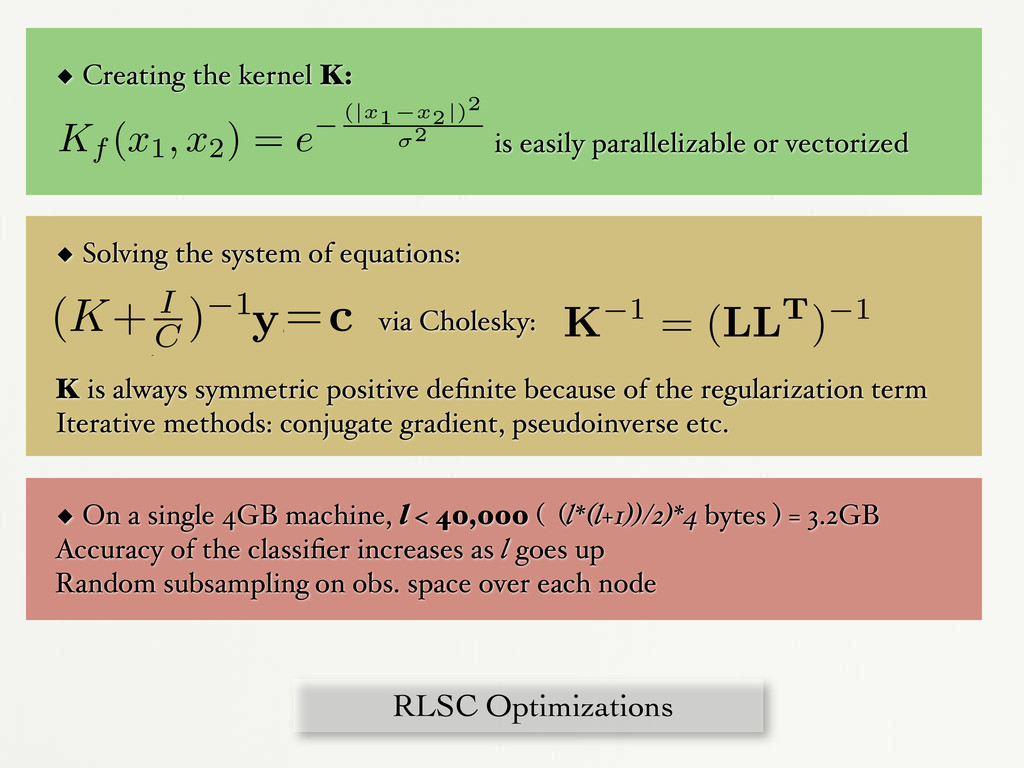
always symmetric positive definite because of the regularization term Iterative methods: conjugate gradient, pseudoinverse etc. RLSC Optimizations n kernel, Kf (x1, x2 ) = e (|x1 x2|)2 2 (1) y| is the conventional Euclidean distance be- points, and is a parameter we keep at 0.5. f (x1, x2 ) = e 2 (1) meter we keep at 0.5. an RLSC system consists of solving the equations (K + I C ) c = y , (2) r-supplied regularization constant. The ued classification function f is f(x) = X i=1 ciK(x, xi ). (3) P(an ) in fined as even in th Now w threshold P(at ) gr manner w scoring c or unimp 6 Lin Disc real-valued classification function f is f(x) = X i=1 ciK(x, xi ). (3) al property of RLSC is that if we store the in- rix (K+ I C ) 1, then for a new right-hand side y , ompute the new c via a simple matrix multipli- his allows us to compute new classifiers (after the data and storing it in memory) on the fly le matrix multiplications. luation for a “Query-by-Description” Task te our connection-finding system, we compute or un 6 L D Given our m terms mode senso ing a hear terms datio on f is (3) we store the in- ght-hand side y , matrix multipli- classifiers (after mory) on the fly ription” Task em, we compute or unimportant. 6 Linguistic Experts for Pa Discovery Given a set of ‘grounded’ single ter our method for uncovering parameter terms and learning the knobs to vary model states that certain knowledge sensory input or intrinsic knowledge ing a ‘linguistic expert.’ If we hear hear ‘quiet’ audio, we would need terms are antonymially related befo dation space between them. Kf (x1, x2 ) = e 2 (1) parameter we keep at 0.5. ning an RLSC system consists of solving the ear equations (K + I C ) c = y , (2) user-supplied regularization constant. The -valued classification function f is f(x) = X i=1 ciK(x, xi ). (3) P(an fined even No thresh P(at mann scorin or un 6 L D o be computed in half the operations over Gaussian elimin ation only requires the lower triangle of the matrix to be st kernel matrix K (which by definition is symmetric positive makes it fully definite) is K 1 = (LLT) 1 where L was derived from the Cholesky decomposition. The ithms for both computing the Cholesky decomposition in pl matrix and also the inverse of the Cholesky factorization avai n our implementations, we use the single precision LAPACK nverse (SPPTRI) on a packed lower triangular matrix. This 2 ◆ Creating the kernel K: is easily parallelizable or vectorized ◆ On a single 4GB machine, l < 40,000 ( (l*(l+1))/2)*4 bytes ) = 3.2GB Accuracy of the classifier increases as l goes up Random subsampling on obs. space over each node
Dangerous 0% Gloomy 29% Fictional 0% Unplugged 30% Magnetic 0% Acoustic 23% Pretentious 1% Dark 17% Gator 0% Female 32% Breaky 0% Romantic 23% Sexy 1% Vocal 18% Wicked 0% Happy 13% Lyrical 0% Classical 27% Worldwide 2% Baseline = 0.14% [Whitman and Ri.in 2002] ◆ Collect all terms through CM as ground truth against corresponding artist feature space -- artist (broad) level! ◆ Evaluation: on a held out test set of audio (with known labels), how well does each classifier predict its label? ◆ In evaluation model, bias is countered: Accuracy of positive association times accuracy of negative association = “P(a) overall accuracy”
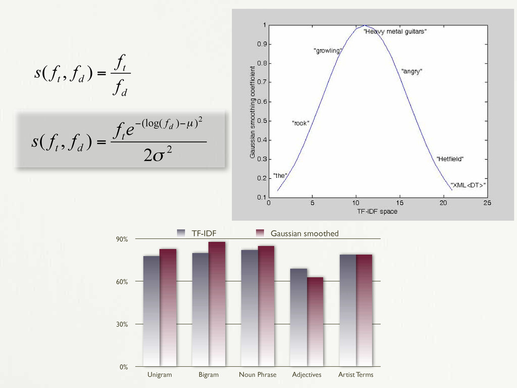
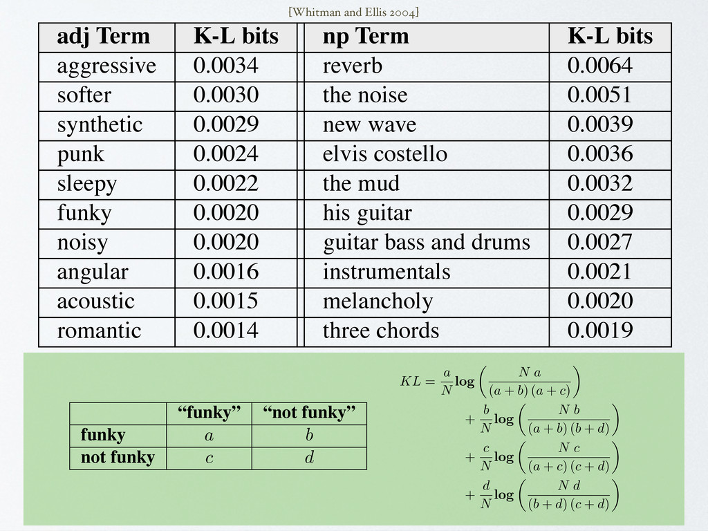
reverb 0.0064 softer 0.0030 the noise 0.0051 synthetic 0.0029 new wave 0.0039 punk 0.0024 elvis costello 0.0036 sleepy 0.0022 the mud 0.0032 funky 0.0020 his guitar 0.0029 noisy 0.0020 guitar bass and drums 0.0027 angular 0.0016 instrumentals 0.0021 acoustic 0.0015 melancholy 0.0020 romantic 0.0014 three chords 0.0019 Table 2. Selected top-performing models of adjective and noun phrase terms used to predict new reviews of music with their corresponding bits of information from the K-L distance measure. [Whitman and Ellis 2004] random guessing is: KL = a N log ✓ N a (a + b) (a + c) ◆ + b N log ✓ N b (a + b) (b + d) ◆ + c N log ✓ N c (a + c) (c + d) ◆ + d N log ✓ N d (b + d) (c + d) ◆ (3) if P(ap ) is the overall positive accuracy (i.e. given an audio frame, the probability that a positive association to a term is predicted) and P(an ) indicates overall nega- tive accuracy, P(a) is defined as P(ap )P(an ). This mea- sure gives us a tangible feeling for how our term mod- els are working against the held out test set and is use- ful for grounded term prediction and the review trimming experiment below. However, to rigorously evaluate our term model’s performance in a review generation task, we note that this value has an undesirable dependence on the prior probability of each label and rewards term classi- fiers with a very high natural df, often by chance. Instead, for this task we use a model of relative entropy, using the Kullback-Leibler (K-L) distance to a random-guess prob- ability distribution. We use the K-L distance in a two-class problem de- scribed by the four trial counts in a confusion matrix: “funky” “not funky” funky a b not funky c d
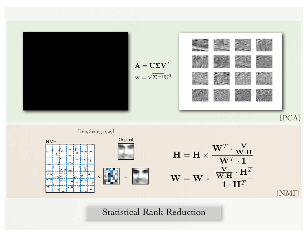
! Original = [Lee, Seung 1999] where is a per-element multiply. The divergence measure here is fo creasing given the following two update rules: H = H WT · V W·H WT · 1 W = W V W·H · HT 1 · HT where 1 is a m n matrix of all 1. 6.2.6 Evaluation using Artist Identification w of a matrix A when Aw = w. ( are the eigenvalues: is an eigenvalue if and only if det(A I) = 0.) We use the singular value decomposition (SVD) [33] to compute the eigenvectors and eigenvalues: A = U VT (6.3) Here, if A is of size m ⇥ n, U is the left singular matrix composed of the singular vectors of size m ⇥ n, V is the right singular matrix matrix of size n ⇥ n, and is a diagonal matrix of the singular values ⇥k . The highest singular value will be in the upper left of the diagonal matrix and in descending order from the top-left. For the covariance matrix input of AAT , U and VT will be equivalent for the non-zero eigenvalued vectors. To reduce rank of the observation matrix A we simply choose the top r vectors of U and the top r singular values in . To compute a weight matrix w from the decomposition we multiply our (cropped) eigenvectors by a scaled version of our (cropped) singular values: [74] w = 1UT (6.4) This w will now be of size r ⇥ m. To project your original data (or new data) through the weight matrix you simply multiply w by A, resulting in a whitened and rank re- duced matrix f of size r⇥n. To ‘resynthesize’ rank reduced matrices projected through w you first compute w 1 and multiply this new iw by f. The intuition behind PCA is to reduce the dimensionality of an observation set; by Here, if A is of size m ⇥ n, U is the left singular matrix composed of the singular vectors of size m ⇥ n, V is the right singular matrix matrix of size n ⇥ n, and is a diagonal matrix of the singular values ⇥k . The highest singular value will be in the upper left of the diagonal matrix and in descending order from the top-left. For the covariance matrix input of AAT , U and VT will be equivalent for the non-zero eigenvalued vectors. To reduce rank of the observation matrix A we simply choose the top r vectors of U and the top r singular values in . To compute a weight matrix w from the decomposition we multiply our (cropped) eigenvectors by a scaled version of our (cropped) singular values: [74] w = 1UT (6.4) This w will now be of size r ⇥ m. To project your original data (or new data) through the weight matrix you simply multiply w by A, resulting in a whitened and rank re- duced matrix f of size r⇥n. To ‘resynthesize’ rank reduced matrices projected through w you first compute w 1 and multiply this new iw by f. The intuition behind PCA is to reduce the dimensionality of an observation set; by ordering the eigenvectors needed to regenerate the matrix and ‘trimming’ only the top r, the experimenter can choose the rate of lossy compression. The compression is achieved through analysis of the correlated dimensions so that dimensions that move in the same direction are minimized. Geometrically, the SVD (and, by extension, PCA) is explained as the top r best rotations of your input data space so that variance between the dimensions are maximized. 6.2.5 NMF Non-negative matrix factorization (NMF) [44] is a matrix decomposition that enforces a positivity constraint on the bases. Given a positive input matrix V of size m ⇥ n, it is factorized into two matrices W of size m ⇥ r and H of size r ⇥ n, where r ⇤ m. The error of ⇧W· H⌃ ⌅ V is minimized. The advantage of the NMF decomposition is that both H and W are non-negative, which is thought to force the decomposition [PCA] [NMF]
with the precise positions of the detected components relative to the upper left corner of the 58 58 window. Overall we have three values per component classifier that are propagated to the combination clas- sifier: the maximum output of the component classifier and the - image coordinates of the maximum. 3. For each component k, determine its maximum output within a search region and its location: Combination classifier: Linear SVM Combination classifier: Linear SVM Left Eye expert: Linear SVM Left Eye expert: Linear SVM . . . 1. Shift 58x58 window over input image *Outputs of component experts: bright intensities indicate high confidence. 2. Shift component experts over 58x58 window 4. Final decision: face / background ) , , ( 14 14 14 Y X O ) , , ,..., , , ( 14 14 14 1 1 1 Y X O Y X O Nose expert: Linear SVM Nose expert: Linear SVM Mouth expert: Linear SVM Mouth expert: Linear SVM . . . * * * ) , , ( 1 1 1 Y X O ) , , ( k k k Y X O ) , , ( k k k Y X O Figure 2: System overview of the component-based classifier. [Heisele, Serre, Pontil, Vetter, Poggio 2001]
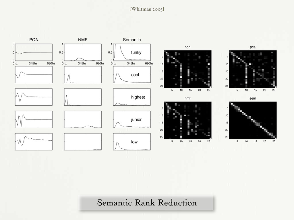
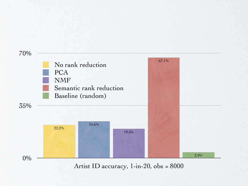
0 2 PCA 0hz 345hz 690hz 0 0.5 1 NMF 0hz 345hz 690hz 0 0.5 1 Semantic funky cool highest junior low Figure 1: Comparison of the top five bases for each type of de- composition, trained from a set of five second power spectral den- sity frames. The PCA weights aim to maximize variance, the NMF weights try to find separable additive parts, and the semantic weights map the best possible labels to the generalized observa- tions. 2003 IEEE Workshop on Applications of Signal Processing to Audio and Acoust non 5 10 15 20 25 5 10 15 20 25 pca 5 10 15 20 25 5 10 15 20 25 nmf 5 10 15 20 25 5 10 15 20 25 sem 5 10 15 20 25 5 10 15 20 25 Figure 3: Confusion matrices for the four experiments. Top: no dimensionality reduction and PCA with r = 10. Bottom: NMF with r = 10 and semantic rank reduction with r = 10. Lighter points indicate that the examples from artists on the x-axis were thought to be by artists on the y-axis. training across the board, with perhaps the NMF hurting the accu- racy versus not having an reduced rank representation at all. For the test case, results widely vary. PCA shows a slight edge over no reduction in the per-observation metric while NMF appears to hurt [Whitman 2003] Semantic Rank Reduction
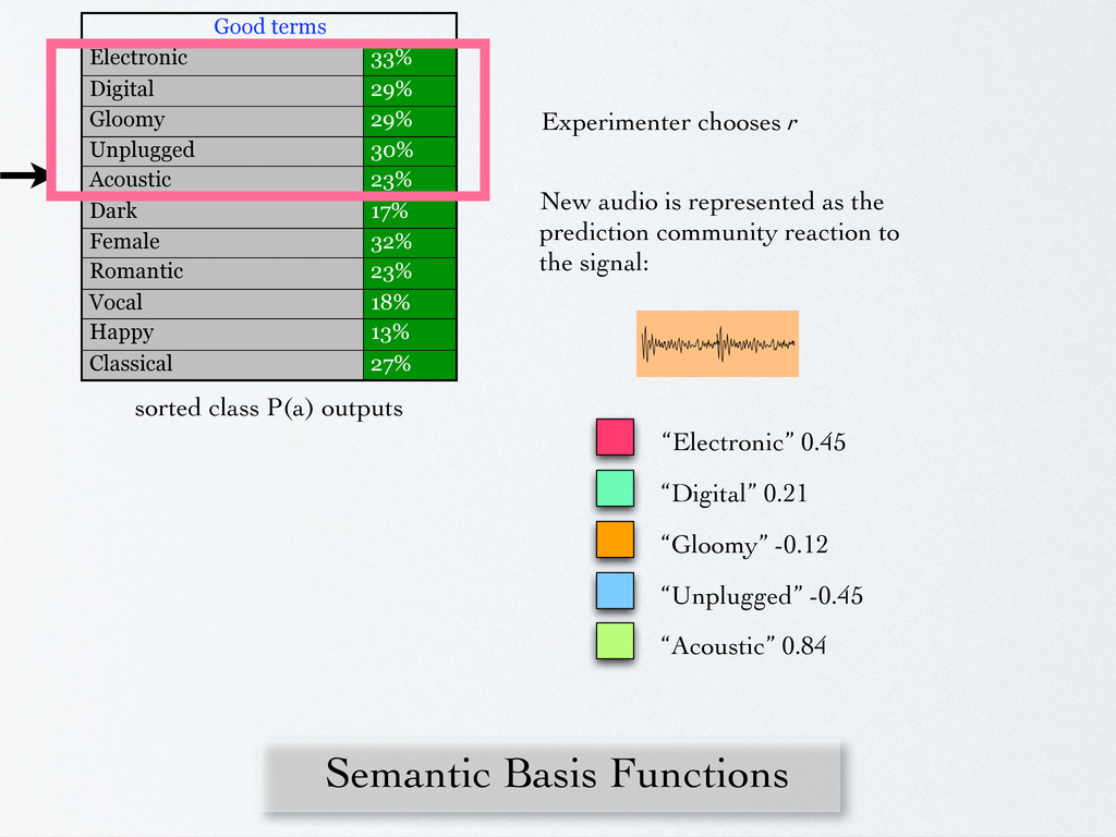
✓ ✓ ✓ ✓ ✓ ✓ community metadata “What the community thinks” Electronic 33% Digital 29% Gloomy 29% Unplugged 30% Acoustic 23% Dark 17% Female 32% Romantic 23% Vocal 18% Happy 13% Classical 27% sorted class P(a) outputs “What are the most important things to a community”
29% Unplugged 30% Acoustic 23% Dark 17% Female 32% Romantic 23% Vocal 18% Happy 13% Classical 27% sorted class P(a) outputs Experimenter chooses r New audio is represented as the prediction community reaction to the signal: “Electronic” 0.45 “Digital” 0.21 “Gloomy” -0.12 “Unplugged” -0.45 “Acoustic” 0.84
of a set of c artists / classes, with training data for each, how many of a set of n songs can be placed in the right class in testing? ◆ Album effect - Learning producers instead of musical content ◆ Time-aware - “Madonna” problem ◆ Data density / overfitting - Sensitive to rate of feature, amount of data per class ◆ Features or learning?
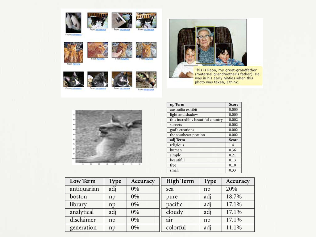
30 40 50 60 70 80 90 100 np Term Score austrailia exhibit 0.003 light and shadow 0.003 this incredibly beautiful country 0.002 sunsets 0.002 god’s creations 0.002 the southeast portion 0.002 adj Term Score religious 1.4 human 0.36 simple 0.21 beautiful 0.13 free 0.10 small 0.33 Figure 7-3: Top terms for community metadata vectors associated with the image at left. informed by the probabilities p(i) of each symbol i in X. More ‘surprising’ symbols in a message need more bits to encode as they are less often seen. This equation com- monly gives a upper bound for compression ratios and is often studied from an artistic standpoint. [54] In this model, the signal contains all the information: its significance is defined by its self-similarity and redundancy, a very absolutist view. However, we in- tend instead to consider the meaning of those bits, and by working with other domains, different packing schemes, and methods for synthesizing new data from these signifi- 10 20 30 40 50 60 70 80 100 beautiful 0.13 free 0.10 small 0.33 Figure 7-3: Top terms for community metadata vectors associated with the image at left. informed by the probabilities p(i) of each symbol i in X. More ‘surprising’ symbols in a message need more bits to encode as they are less often seen. This equation com- monly gives a upper bound for compression ratios and is often studied from an artistic standpoint. [54] In this model, the signal contains all the information: its significance is defined by its self-similarity and redundancy, a very absolutist view. However, we in- tend instead to consider the meaning of those bits, and by working with other domains, different packing schemes, and methods for synthesizing new data from these signifi- cantly semantically-attached representations we hope to bring meaning back into the notion of information. 7.2.1 Images and Video Low Term Type Accuracy antiquarian adj 0% boston np 0% library np 0% analytical adj 0% disclaimer np 0% generation np 0% High Term Type Accuracy sea np 20% pure adj 18.7% pacific adj 17.1% cloudy adj 17.1% air np 17.1% colorful adj 11.1%
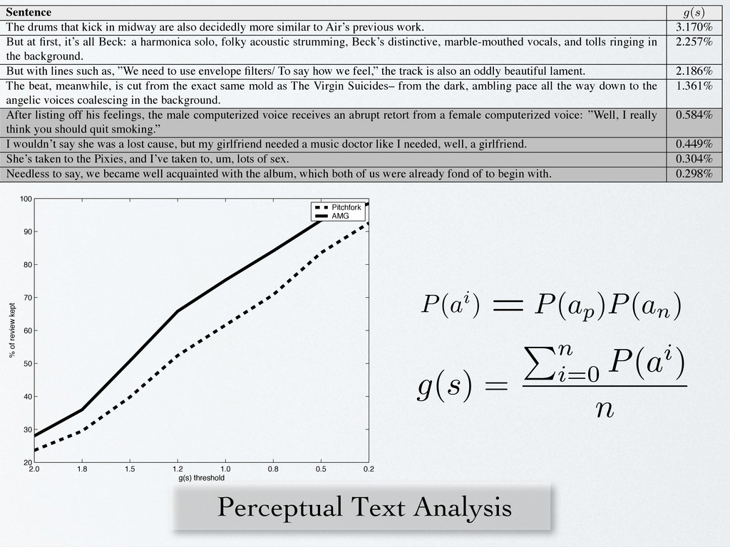
decidedly more similar to Air’s previous work. 3.170% But at first, it’s all Beck: a harmonica solo, folky acoustic strumming, Beck’s distinctive, marble-mouthed vocals, and tolls ringing in the background. 2.257% But with lines such as, ”We need to use envelope filters/ To say how we feel,” the track is also an oddly beautiful lament. 2.186% The beat, meanwhile, is cut from the exact same mold as The Virgin Suicides– from the dark, ambling pace all the way down to the angelic voices coalescing in the background. 1.361% After listing off his feelings, the male computerized voice receives an abrupt retort from a female computerized voice: ”Well, I really think you should quit smoking.” 0.584% I wouldn’t say she was a lost cause, but my girlfriend needed a music doctor like I needed, well, a girlfriend. 0.449% She’s taken to the Pixies, and I’ve taken to, um, lots of sex. 0.304% Needless to say, we became well acquainted with the album, which both of us were already fond of to begin with. 0.298% Table 3. Selected sentences and their g(s) in a review trimming experiment. From Pitchfork’s review of Air’s “10,000 Hz Legend.” 2.0 1.8 1.5 1.2 1.0 0.8 0.5 0.2 20 30 40 50 60 70 80 90 100 g(s) threshold % of review kept Pitchfork AMG lation we established that a random association of these two datasets gives a correlation coefficient of magnitude smaller than r = 0.080 with 95% confidence. Thus, these results indicate a very significant correlation between the automatic and ground-truth ratings. The Pitchfork model did not fare as well with r = 0.127 (baseline of r = 0.082 with 95% confidence.) Fig- ure 1 shows the scatter plot/histograms for each experi- ment; we see that the audio predictions are mainly bunched around the mean of the ground truth ratings and have a much smaller variance. Visually, it is hard to judge how well the review information has been captured. However, the correlation values demonstrate that the automatic anal- ysis is indeed finding and exploiting informative features. Perceptual Text Analysis 2.0 1.8 1.5 1.2 1.0 0.8 0.5 0.2 20 30 40 50 60 70 80 90 100 g(s) threshold % of review kept Pitchfork AMG erstand- without ere cho- e testing t term’s d in re- etting a e vector grounded term models for insights into th description and develop a ‘review trimmin summarizes reviews and retains only the m content. The trimmed reviews can then b ther textual understanding systems or read listener. To trim a review we create a grounding ated on a sentence s of word length n, g(s) = Pn i=0 P(ai) n where a perfectly grounded sentence (in wh tive qualities of each term on new music h a large defined observa- associ- el-space ulariza- esultant rom the or each esenting hat term a ‘ma- xamples testing gram matrix and check each learned c again audio frame in the test set. We used two separate evaluation techniques t the strength of our term predictions. One metric is sure classifier performance with the recall produc if P(ap ) is the overall positive accuracy (i.e. gi audio frame, the probability that a positive asso to a term is predicted) and P(an ) indicates overal tive accuracy, P(a) is defined as P(ap )P(an ). Th sure gives us a tangible feeling for how our term els are working against the held out test set and ful for grounded term prediction and the review tri experiment below. However, to rigorously evalu term model’s performance in a review generation t note that this value has an undesirable dependence ich nd- out ho- ing m’s re- g a ctor lso n a os- mother loves this album.” We look to the success of our grounded term models for insights into the musicality of description and develop a ‘review trimming’ system that summarizes reviews and retains only the most descriptive content. The trimmed reviews can then be fed into fur- ther textual understanding systems or read directly by the listener. To trim a review we create a grounding sum term oper- ated on a sentence s of word length n, g(s) = Pn i=0 P(ai) n (4) where a perfectly grounded sentence (in which the predic- tive qualities of each term on new music has 100% preci- sion) is 100%. This upper bound is virtually impossible in a grammatically correct sentence, and we usually see g(s) of {0.1% .. 10%}. The user sets a threshold and the sys- tem simply removes sentences under the threshold. See Kf (x1, x2 ) = e 2 re is a parameter we keep at 0.5. hen, training an RLSC system consists of em of linear equations (K + I C ) c = y , re C is a user-supplied regularization con lting real-valued classification function f
full-length is their most experimental effort to date -- fractured melodies and dub-like rhythms collide in a noisy atmosphere rich in detail, adorned with violins, trumpet, severe phasing effects, and even a typewriter. - Jason Ankeny [Arovane, “Tides”] The homeless lady who sits outside the yuppie coffee bar on the corner of my street assures passers-by that the end is coming. I think she’s desperate to convey her message. Though the United States is saber-rattling with the People’s Republic of China, it seems that everyone has overcome their millennial tension, and the eve of destruction has turned to a morning of devil-may-care optimism. Collectively, we’re overjoyed that, without much effort or awareness, we kicked the Beasťs ass. The Beast, as prophesied by some locust-muncher out in the Negev Desert thousands of years ago, was supposed to arrive last year and annihilate us before being mightily smote by our Lord and Savior Jesus Christ. I missed this. Living as I do in America’s capital, the seat of iniquity and corruption, I should have had ring-side seats to the most righteous beatdown of all time. I even missed witnessing the Rapture, the faithfuľs assumption to the right hand of God that was suppose to occur just before Satan’s saurian shredded all of creation.... [it goes o% like this for a while] - Paul Cooper Perceptual Text Analysis 0.862 4.15
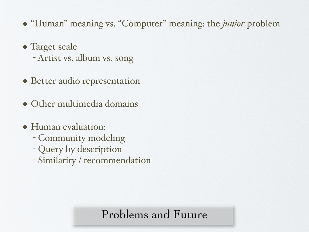
Target scale - Artist vs. album vs. song ◆ Better audio representation ◆ Other multimedia domains ◆ Human evaluation: - Community modeling - Query by description - Similarity / recommendation Problems and Future
Keith, Michael Casey, Judy, Mike Mandel, Wei, Victor, John, Nyssim, Rebecca, Kristie, Tamara Hearn. Dan Ellis & Columbia; Adam Berenzweig, Ani Nenkova, Noemie Elhadad. Deb Roy. Ben Recht, Ryan Ri.in, Jason, Mary, Tristan, Rob A, Hugo S, Ryan McKinley, Aggelos, Gemma & Ayah & Tad & Limor, Hyun, Cameron, Peter G. Dan P., Chris C, Dan A, Andy L., Barbara, Push, Beth Logan. ex-NECI: Steve Lawrence, Gary Flake, Lee Giles, David Waltz. Kelly Dobson, Noah Vawter, Ethan Bordeaux, Scott Katz, Tania & Ruth, Lauren Kroiz. Drew Daniel, Kurt Ralske, Lukasz L., Douglas Repetto. Bruce Whitman, Craig John and Keith Fullerton Whitman. Stanley and Albert (mules), Wilbur (cat), Sara Whitman and Robyn Belair. Sofie Lexington Whitman:
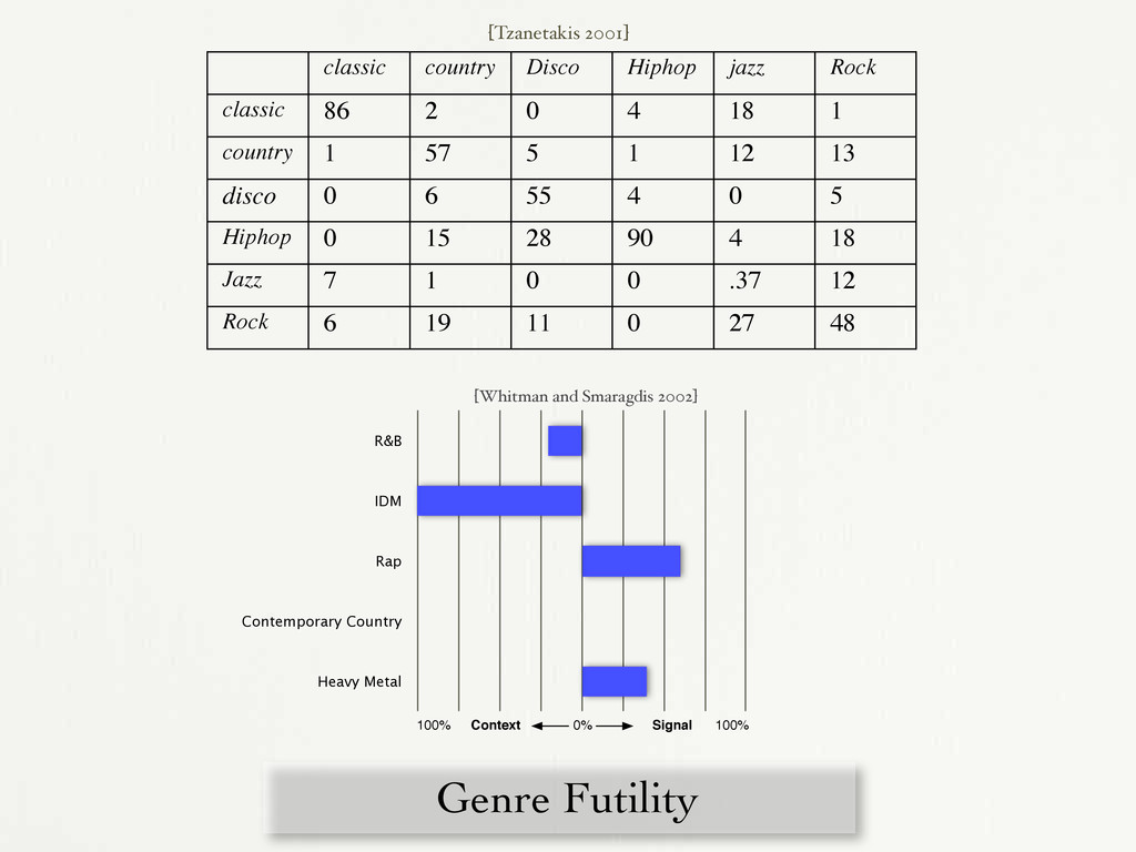
Reviews.” In Proceedings of ISMIR 2004 - 5th International Conference on Music Information Retrieval. October 10-14, 2004, Barcelona, Spain. Berenzweig, Adam, Beth Logan, Daniel Ellis, Brian Whitman. “A Large Scale Evaluation of Acoustic and Subjective Music Similarity Measures.” Computer Music Journal, Summer 2004, 28(2), pp 63-76. Whitman, Brian. “Semantic Rank Reduction of Music Audio.” In Proceedings of the 2003 Workshop on Applications of Signal Processing to Audio and Acoustics (WASPAA). 19-22 October 2003, New Paltz, NY. pp135-138 Whitman, Brian, Deb Roy, and Barry Vercoe. “Learning Word Meanings and Descriptive Parameter Spaces from Music.” in Proceedings of the HLT- NAACL03 workshop on Learning Word Meaning from Non-Linguistic Data. 26 -31 May 2003, Edmonton, Alberta, Canada. Whitman, Brian and Ryan Ri.in. “Musical Query-by-Description as a Multiclass Learning Problem.” In Proceedings of the IEEE Multimedia Signal Processing Conference. 8-11 December 2002, St. Thomas, USA. Ellis, Daniel, Brian Whitman, Adam Berenzweig and Steve Lawrence. “The Quest For Ground Truth in Musical Artist Similarity.” In Proceedings of the 3rd International Conference on Music Information Retrieval. 13-17 October 2002, Paris, France. Whitman, Brian and Paris Smaragdis. “Combining Musical and Cultural Features for Intelligent Style Detection.” In Proceedings of the 3rd International Conference on Music Information Retrieval. 13-17 October 2002, Paris, France. Whitman, Brian and Steve Lawrence (2002). “Inferring Descriptions and Similarity for Music from Community Metadata.” In “Voices of Nature,” Proceedings of the 2002 International Computer Music Conference. pp 591-598. 16-21 September 2002, Göteborg, Sweden.
![[M.I.A. “Galang” from Arular, XL Recordings] 0 75 150 225](https://files.speakerdeck.com/presentations/320b12709241013049086ed34696e943/slide_5.jpg)
![[Mueller] [Miller] [All Media Guide]](https://files.speakerdeck.com/presentations/320b12709241013049086ed34696e943/slide_26.jpg)
![[Duygulu, Barnard, Freitas, Forsyth 2002] sea sky sun waves cat](https://files.speakerdeck.com/presentations/320b12709241013049086ed34696e943/slide_27.jpg)
![[All Media Guide]](https://files.speakerdeck.com/presentations/320b12709241013049086ed34696e943/slide_28.jpg)
![Webtext [Whitman, Lawrence 2002] Search for target context (artistname, songname)](https://files.speakerdeck.com/presentations/320b12709241013049086ed34696e943/slide_32.jpg)
![the visual cortex [8]. We also provide the combination classifier](https://files.speakerdeck.com/presentations/320b12709241013049086ed34696e943/slide_52.jpg)
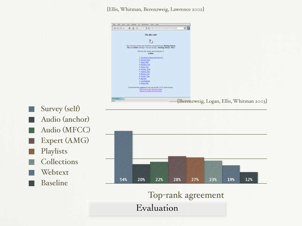
![[Berenzweig, Ellis, Lawrence 2002] [Apple 2003]](https://files.speakerdeck.com/presentations/320b12709241013049086ed34696e943/slide_53.jpg)
![[June of 44, “Four Great Points”] June of 44's fourth](https://files.speakerdeck.com/presentations/320b12709241013049086ed34696e943/slide_61.jpg)