Hertie Data Science Lab Summer School: Text as Data

Transcript

1. T D : S S William Lowe Hertie School July ,
2. ... From Padua ( ) P → Text as data → Document classi cation → Models for topicful documents → Documents in space Will Lowe . .
3. Y → Dr William Lowe conjugateprior@gmail.com → Senior Research Scientist Data Science Lab, Hertie School → e emergency backup instructor “in case of emergency break class” B → Dr Olga Gasparyan → Huy Ngoc Dang → Bruno Ponne Will Lowe . .
4. Y → Dr William Lowe conjugateprior@gmail.com → Senior Research Scientist Data Science Lab, Hertie School → e emergency backup instructor “in case of emergency break class” B → Dr Olga Gasparyan → Huy Ngoc Dang → Bruno Ponne M → Practical exercises are available as zip le on the course page → Each session has a folder → Each folder contains an RStudio project le (click to launch) → *.html is a code walk-through → *.R is the code → You’ll never need to change the working directory Will Lowe . .
5. Broad approaches to studying text data → Just read it and think a bit, e.g. op-eds, punditry, kremlinology, grand strategy, etc. → Discourse Analysis → Natural Language Processing (NLP) → Text as Data (TADA) the last two are, broadly, Computational Linguistics, but with a di erent focus Will Lowe . .
6. Although discourse analysis can be applied to all areas of research, it cannot be used with all kinds of theoretical framework. Crucially, it is not to be used as a method of analysis detached from its theoretical and methodological foundations. Each approach to discourse analysis that we present is not just a method for data analysis, but a theoretical and method- ological whole - a complete package. [...] In discourse and analysis theory and method are intertwined and researchers must accept the basic philosophical premises in order to use discourse analysis as their method of empirical study. (Jørgensen & Phillips, ) Apparent di erences are theoretical. e important di erence for us is that → Discourse analysis tightly couples theory and measurement Substantive theory ≠ textual measurement...but they do have implications for one another Will Lowe . .
7. ( ) A typical NLP pipeline → Segmentation / tokenization → Part of Speech (POS) tagging → Parsing → Named Entity Recognition (NER) → Information Extraction (IE) Will Lowe . .
8. ( ) A typical NLP pipeline → Segmentation / tokenization → Part of Speech (POS) tagging → Parsing → Named Entity Recognition (NER) → Information Extraction (IE) President Xi Jinping of China, on his rst state visit to the United States, showed o his familiarity with American history and pop culture on Tuesday night. Will Lowe . .
9. ( ) A typical NLP pipeline → Segmentation / tokenization → Part of Speech (POS) tagging → Parsing → Named Entity Recognition (NER) → Information Extraction (IE) Tools: → Spacy (spacy.io) and accessible from R using {spacyr} → Stanford NLP tools (nlp.stanford.edu) Will Lowe . .
10. : We are the measurement component for social science theory → eory provides the things to be measured → Words and sometimes other things provide the data to measure them → Language agnostic, evidentially behaviourist, structurally indi erent, shamelessly opportunistic → obsessed with counting words If Discourse Analysis o ers close reading, we will o er distant reading Advantages → Scales well → Easy to integrate into existing models → Can guide close reading later Will Lowe . .
11. What are the conditions for the possibility for taking a TADA approach In plainer language: → How could this possibly work? An uncharacteristically dashing Kant Will Lowe . .
12. ere is a message or content that cannot be directly observed, e.g. → the topic of this talk → my position on some political issue → the importance of defence issues to a some political party and behaviour, including linguistic behaviour, e.g. → yelling, writing, lecturing which can be directly observed. Although language can do things directly – inform, persuade, demand, threaten, (Austin, ) – we’ll focus on its signal properties: expressed message and its words... Will Lowe . .
13. To communicate a message θ (or Z) to a producer (the speaker or writer) generates words of di erent kinds in di erent quantities For models: the generative mode ... Tiber ow with much θ blood ... To understand a message the consumer (the hearer, reader, coder) uses those words to reconstruct the message For models: the discriminative mode ... Tiber ow with much θ blood ... Will Lowe . .
14. : We’ll represent the sample of N words in a ‘plate’ W N θ And usually use Z as a categorical ’message’ and θ as a continuous one Will Lowe . .
15. : We’ll represent the sample of N words in a ‘plate’ W N θ And usually use Z as a categorical ’message’ and θ as a continuous one We can read this several ways: → causal: θ causes those words to be generated → statistical (general): ere exists a conditional distribution of W given θ → statistical (measurement): Ws are conditionally independent given θ → practical: Somewhere in the model is a table relating θ to W Will Lowe . .
16. is process is → stable (Grice, ; Searle, ) → conventional (Lewis, / ) → disruptible (Riker et al., ) → empirically underdetermined (Davidson, ; Quine, ) How to model this without having to solve the problems of linguistics (psychology, politics) rst? Rely on: → instrumentality → re exivity → randomness Will Lowe . .
17. (Urban dictionary, July ) e di erence between → X means Y → X is used to mean Y Will Lowe . .
18. : Politicians are o en nice enough to talk as if they really do communicate this way My theme here has, as it were, four heads. [...] e rst is articulated by the word “oppor- tunity” [...] the second is expressed by the word “choice” [...] the third theme is summed up by the word “strength” [and] my fourth theme is expressed well by the word “renewal”. (Note however, these words occur , , , and times in words) Will Lowe . .
19. : Politicians are o en nice enough to talk as if they really do communicate this way My theme here has, as it were, four heads. [...] e rst is articulated by the word “oppor- tunity” [...] the second is expressed by the word “choice” [...] the third theme is summed up by the word “strength” [and] my fourth theme is expressed well by the word “renewal”. (Note however, these words occur , , , and times in words) A couple months ago we weren’t expected to win this one, you know that, right? We weren’t...Of course if you listen to the pundits, we weren’t expected to win too much. And now we’re winning, winning, winning the country – and soon the country is going to start winning, winning, winning. Will Lowe . .
20. Will Lowe . .
21. Quantitative text analysis works best when language usage is stable, conventionalized, and instrumental. Implicitly, that means institutional language, e.g. → courts → legislatures → op-eds → nancial reporting Institution-speci city analyses inevitably create comparability problems, e.g. between → upper vs lower chamber vs parliamentary hearings → bureaucracy vs lobby groups (Klüver, ) → European languages (Proksch et al., ) Will Lowe . .
22. We are going to design instruments to measure θ and are going to assume that the θ → W relationships are institutionally stable What if they aren’t? Will Lowe . .
23. We are going to design instruments to measure θ and are going to assume that the θ → W relationships are institutionally stable What if they aren’t? Will Lowe . .
24. Google u trends. Predictive, until it wasn’t. (Lazer et al., ) Will Lowe . .
25. Sometimes actors are happy to solve comparability problems for us, e.g. → Lower court opinions (Corley et al., ) or Amicus briefs (Collins et al., ) embedded in Supreme Court opinions → ALEC model bills embedded in state bills (Garrett & Jansa, ) A perfect jobs for text-reuse algorithms... Will Lowe . .
26. : Why randomness? → You almost never say exactly the same words twice, even when you haven’t changed your mind about the message. → so words are the result of some kind of sampling process. → We model this process as random because we don’t know or care about all the causes of variation Will Lowe . .
27. : Why randomness? → You almost never say exactly the same words twice, even when you haven’t changed your mind about the message. → so words are the result of some kind of sampling process. → We model this process as random because we don’t know or care about all the causes of variation Note: → What is ‘signal’ and what is ‘noise’ is relative to your and the sources’ purposes Will Lowe . .
28. : Why randomness? → You almost never say exactly the same words twice, even when you haven’t changed your mind about the message. → so words are the result of some kind of sampling process. → We model this process as random because we don’t know or care about all the causes of variation Note: → What is ‘signal’ and what is ‘noise’ is relative to your and the sources’ purposes Also, we’re all secretly Bayesians Will Lowe . .
29. What do we know about words as data? ey are di cult → High dimensional → Sparsely distributed (with skew) → Not equally informative Will Lowe . .
30. Example: Conservative party manifesto compared to other parties over four elections: → High dimensional. word types (adult native english speakers know - , ) → Sparse. at’s about . % the , word types deployed over these elections → Skewed. Of these words appeared exactly once and the most frequent word times Will Lowe . .
31. Example: Conservative party manifesto compared to other parties over four elections: → High dimensional. word types (adult native english speakers know - , ) → Sparse. at’s about . % the , word types deployed over these elections → Skewed. Of these words appeared exactly once and the most frequent word times More generally: the Zipf-Mandelbrot law (Mandelbrot, ; Zipf, ) F(Wi ) ∝ rank(Wi )α where rank(.) is the frequency rank of a word in the vocabulary and α ≈ is is a Pareto distribution in disguise Will Lowe . .
32. 0 5000 10000 15000 20000 0 2500 5000 7500 rank frequency Source Cons 2017 Corpus 1 10 100 1000 10000 1 10 100 1000 10000 rank frequency Source Cons 2017 Corpus See Chater and Brown ( ) on scale invariance. Will Lowe . .
33. More generally: the Heaps-Herdan Law states that the number of word types appearing for the rst time a er n tokens is D(n) = Knβ where K is between and and β ≈ . for English. (All the party manifestos shown here) 1 10 100 1000 1 10 100 1000 10000 tokens word types Will Lowe . .
34. Frequency is inversely proportional to substantive interestingness Word Freq. the and to of we will Top Word Freq. . . . . . rigination Bottom ten Word Freq. people new government support work uk Top ten minus stopwords Will Lowe . .
35. Removing stopwords, while standard in computer science, is not necessarily better... Example: → Standard collections contain, ‘him’, ‘his’, ‘her’ and ‘she’. → Words you’d want to keep when analyzing an abortion debates. Will Lowe . .
36. For large amounts of text summaries are not enough. We need a model to provide assumptions about → equivalence → exchangeability Text as data approaches started o asserting equivalences, and ended up modeling with increasingly sophisticated versions of exchangeability Since ontogeny recapitulates phylogeny, let’s walk through some standard text processing steps, asserting equivalences along the way... Will Lowe . .
37. As I look ahead I am lled with foreboding. Like the Roman I seem to see ‘the river Tiber owing with much blood’...” (Powell, ) Will Lowe . .
38. As I look ahead I am lled with foreboding. Like the Roman I seem to see ‘the river Tiber owing with much blood’...” (Powell, ) index token as i look ahead i am ... index token like the roman i seem to ... Will Lowe . .
39. type count as i look ahead am ... ... token count like the roman i seem to ... ... Will Lowe . .
40. ‘doc’ ‘doc’ type ahead am as i like look roman seem the to ... ... ... is is the notorious bag-of-words or exchangeability assumption Will Lowe . .
41. We have turned a corpus into a contingency table. → Or a term-document / document-term / document-feature matrix, in the lingo ahead am i like look doc ... θdoc doc ... θdoc βahead βam βi βlike βlook Everything you learned in your last categorical data analysis course applies here → except that the parts of primary interest are not observed Will Lowe . .
42. So what are we going to assume about the word counts? Word counts/rates are conditionally Poisson: Wj ∼ Poisson(λj ) E[Wj ] = Var[Wj ] = λj We’ll let model assumptions determine how λ is related to θ → typically generating proportional increases or decreases in λ Will Lowe . .
43. e Poisson assumption implies that for conditional on document length, word counts are Multinomial: Wi . . . WiV ∼ Mult(Wi . . . WiV π . . . πV , Ni ) Here E[W] = Nπ and Cov[Wj , Wk ] = −Ni πjπk Negative covariance is due to the ‘budget constraint’ Ni Will Lowe . .
44. : Statistical models of text deal with (some kinds of) absence as well as presence We will be concerned with two kinds of absence: → Not seeing a word used – a ‘zero count’ → Not seeing a document at all – ‘sample selection’ (roughly overlapping with item vs unit non-response) Will Lowe . .
45. : Not seeing a word used is fairly easy to deal with → Zero counts are just counts that happen to be zero → Absence is informative to the extent it is surprising → Surprise implies expectations, and expectations imply a model Will Lowe . .
46. : Not seeing a document is harder. → What documents could we have seen but did not → What would we have inferred about content had we seen them? Proksch and Slapin ( ) is a formal and treatment of this problem for legislative debate (see also Giannetti & Pedrazzani, ) → institutionally speci c, because sample selection is a research design problem Will Lowe . .
47. Conventionally, text comes in the ‘documents’ and contains ‘words’, but these are terms of art. You choose what is a document → documents → chapters → sections → window contexts → sentences → tweets → responses You choose what is a word → contiguous letters separated by white space → lemmas / stems → bigrams and n-grams → phrases and names → mentions of topics → expressions of positive a ect Anything we can count, really... Will Lowe . .
48. General advice: → Let the substance guide → Keep your options open; whether a model is realistic is relative to purpose Technical constraints: → Some unit choices will enable (or rule out) certain models → Some bags of words are baggier than others Will Lowe . .
49. For each research problem involving text analysis we need to ask: → What structure does θ or Z have? topic, topic proportions, position → What is observed, assumed, and inferred? → relationship between θ or Z and the words? Which direction do we want to model? → Discriminative → Generative D We sometimes see Z or θ and can learn P(θ W . . . WN ) from a corpus. Typically con rmatory G We don’t see Z or θ but can make assumptions about how words are generated from them P(θ W . . . WN ) = P(W . . . WN θ)P(θ) P(W . . . WN ) Typically exploratory Will Lowe . .
50. Z → Text as data approaches to text analyses rely on institutionalized language usage, → ey assume stable meaning-word relations, → You to decide what a document or word is, → Text’s skewed high-dimensional nature is solved by with models → Models may be discriminative or generative Will Lowe . .
51. Every document is on one of K topics / categories We have a labeled ‘training’ sample What are the rest about? Will Lowe . .
52. Two sides of the one technology → Tool for assigning topics to new document on the basis of labeled existing documents → Tool for learning about how documents express topics in words e rst can be a useful research assistant → We want the best classi er you can train. period e second can generate insight → We want the most interpretable parameters Sometimes we can have these together. But not o en... We’ll look at Naive Bayes, an old but serviceable generative model, and its alter ego a purely discriminative model Will Lowe . .
53. D documents, each on topic Z = k of K W Z N θ β K D is model is written generatively → How to generate words in a document on one topic We will → learn these relationships → update our view of θ with new documents Will Lowe . .
54. D documents, each on topic Z = k of K W Z N θ β K D is model is written generatively → How to generate words in a document on one topic We will → learn these relationships → update our view of θ with new documents G : e proportion of documents of topic k is P(Z = k) = θk we have a prior over this en we’ll estimate the probability that topic k generates the ith word βik = P(Wi Z = k, β) Will Lowe . .
55. D documents, each on topic Z = k of K W Z N θ β K D is model is written generatively → How to generate words in a document on one topic We will → learn these relationships → update our view of θ with new documents D Of more interest is the topic of some particular document {W} P(Z = k {W}, β) Infer this reversing the generation process with Bayes theorem Will Lowe . .
56. : Example application: Evans et al. ( ) attempt to → Discriminate the amicus briefs from each side of two a rmative action cases: Regents of the University of California v. Bakke ( ) and Grutter/Gratz v. Bollinger ( ). → Characterize the language used by each side We will label the Plainti as ‘Conservative’ and the Respondents as ‘Liberal’ All told, Bakke included amicus briefs ( for the conservative side and for liberals) and Bollinger received ( conservative and liberal). (Evans et al., ) e four briefs of Plainti s and Respondents formed the ‘training data’ Will Lowe . .
57. e document category is Z ∈ {Lib, Con} P(Z) = θ Prior probability P({W} Z) = j P(Wj Z) e naive part Words are assumed to be generated independently given the category Z P(‘A rmative Action’ Z = ‘Lib’) = P(‘A rmative’ Z = ‘Lib’)P(‘Action’ Z = ‘Lib’) Will Lowe . .
58. e document category is Z ∈ {Lib, Con} P(Z) = θ Prior probability P({W} Z) = j P(Wj Z) e naive part Words are assumed to be generated independently given the category Z P(‘A rmative Action’ Z = ‘Lib’) = P(‘A rmative’ Z = ‘Lib’)P(‘Action’ Z = ‘Lib’) Classi cation here means doing something with P(Z = ‘Lib’ {W}) Strictly speaking, this is just probability estimation; classi cation is a separate decision problem Will Lowe . .
59. P : Estimating P(Z = ‘Lib’) = − P(Z = ‘Con’) is straightforward: → Count the number of ‘Lib’ documents and divide by the total number of documents L Estimating P(Wj Z = ‘Lib’) is also straightforward (though see McCallum & Nigam, ) → Compute the proportion of words in ‘Lib’ training documents that were word j Will Lowe . .
60. P Use Bayes theorem to get the probability of, e.g. an amicus brief being ‘Lib’ given the words inside Will Lowe . .
61. P Use Bayes theorem to get the probability of, e.g. an amicus brief being ‘Lib’ given the words inside P(Z = ‘Lib’ {W}) = ∏j P(Wj Z = ‘Lib’)P(Z = ‘Lib’) ∏j P(Wj Z = ‘Lib’)P(Z = ‘Lib’) + ∏j P(Wj Z = ‘Con’)P(Z = ‘Con’) Oof. It will be easier to look at how much more likely the brief is to be ‘Lib’ than ‘Con’ Will Lowe . .
62. P(Z = ‘Lib’ {W}) P(Z = ‘Con’ {W}) = j P(Wj Z = ‘Lib’) P(Wj Z = ‘Con’) × P(Z = ‘Lib’) P(Z = ‘Con’) Every new word adds a bit of information that re-adjusts the conditional probabilities → Multiply by something greater than one: more ‘Lib’ → Multiply by something less than one: more ‘Con’ Will Lowe . .
63. It’s o en more useful to work with logged ratios of counts and proportions a.k.a. ‘logits’ log( ) ≈ . log( . ) ≈ − . Advantages: → symmetrical → interpretable zero point → proportional / percentage increases and decreases → Psychophysical and decision-theoretic motivations (see Zhang & Maloney, ) → Measurement theoretic motivations (Rasch, IRT, Bradley Terry models etc.) → Makes products into additions Will Lowe . .
64. log P(Z = ‘Lib’ {W}) P(Z = ‘Con’ {W}) = j log P(Wj Z = ‘Lib’) P(Wj Z = ‘Con’) + log P(Z = ‘Lib’) P(Z = ‘Con’) Every new word adds a bit of information that re-adjusts the conditional probabilities Will Lowe . .
65. Example: Naive Bayes with only word class ‘discriminat*’. Assume that liberal and conservative supporting briefs are equally likely (true in the training set) P(Z = ‘Lib’) P(Z = ‘Con’) = and P(W = ‘discriminat*’ Z = ‘Lib’) = ( + ) ( + ) ≈ . P(W = ‘discriminat*’ Z = ‘Con’) = ( + ) ( + ) ≈ . Posterior probability ratio is about to in favour of the document supporting the conservative side Will Lowe . .
66. Will Lowe . .
67. → ere are no identi able uniquely partisan words → but these associations are stable in cases years apart Will Lowe . .
68. Amicus brief from ‘King County Bar Association’ containing words and matches to disciminat*. that "the state shall not [discriminate] against, or grant preferential treatment the lingering effects of racial [discrimination] against minority groups in this remedy the effects of societal [discrimination]. Another four Justices (Stevens that "the state shall not [discriminate] against, or grant preferential treatment Will Lowe . .
69. e posterior probability of a document being liberal is P(Z = ‘Lib’ {W}) = ∏j P(Wj Z = ‘Lib’)P(Z = ‘Lib’) ∏j P(Wj Z = ‘Lib’)P(Z = ‘Lib’) + ∏ P(Wj Z = ‘Con’)P(Z = ‘Con’) but let’s do a little rearranging Will Lowe . .
70. e posterior probability of a document being liberal is P(Z = ‘Lib’ {W}) = ∏j P(Wj Z = ‘Lib’)P(Z = ‘Lib’) ∏j P(Wj Z = ‘Lib’)P(Z = ‘Lib’) + ∏ P(Wj Z = ‘Con’)P(Z = ‘Con’) but let’s do a little rearranging P(Z = Lib {W}) = + exp(−η) η = log P(Z = ‘Lib’) P(Z = ‘Con’) + j log P(Wj Z = ‘Lib’) P(Wj Z = ‘Con’) which might remind you of a model you’ve seen before... Will Lowe . .
71. Say W is ‘discriminate’ and it occurs Cdiscriminate = times in some document then we’ll then add lots of βdiscriminate = log P(discriminate Z = ‘Lib’) P(discriminate Z = ‘Con’) or Cdiscriminate × βdiscriminate Will Lowe . .
72. Say W is ‘discriminate’ and it occurs Cdiscriminate = times in some document then we’ll then add lots of βdiscriminate = log P(discriminate Z = ‘Lib’) P(discriminate Z = ‘Con’) or Cdiscriminate × βdiscriminate so our nal discrimination function has the form P(Z = ‘Lib’ {W}) = + exp(−η) η = β + C β + C β + . . . + CV βV is is a logistic regression on the document term matrix (Jordan, ) a.k.a. ‘Maxent’. Will Lowe . .
73. Naive Bayes and Logistic Regression are in some sense the ‘same model’ → As it happens, any exponential family choice for P(Wj Z) has logistic regression as its discriminative model Will Lowe . .
74. Naive Bayes and Logistic Regression are in some sense the ‘same model’ → As it happens, any exponential family choice for P(Wj Z) has logistic regression as its discriminative model For easy illumination but weaker classi cation performance: → Naive Bayes For less illumination but stronger classi cation performance: → Regularized logit → or Random forests, Support Vector Machines, etc. Will Lowe . .
75. W Z N θ β K D Naive Bayes (generative) W Z N θ β K D σ Logistic regression (discriminative) Will Lowe . .
76. Logistic regression is more focused → No interest in P(W . . . WV ). Words can be conditionally independent, or not. It just wants the decision boundary Will Lowe . .
77. Logistic regression is more focused → No interest in P(W . . . WV ). Words can be conditionally independent, or not. It just wants the decision boundary Intuition: p(x|C1 ) p(x|C2 ) x class densities 0 0.2 0.4 0.6 0.8 1 0 1 2 3 4 5 x p(C1 |x) p(C2 |x) 0 0.2 0.4 0.6 0.8 1 0 0.2 0.4 0.6 0.8 1 1.2 Will Lowe . .
78. But slower and hungrier → β estimates converge at rate N, compared to log N for Naive Bayes’ probability ratios Will Lowe . .
79. But slower and hungrier → β estimates converge at rate N, compared to log N for Naive Bayes’ probability ratios Needs extra guidance to work well → We t Naive Bayes on four documents → Logistic regression will requires regularization for that to work Some natural regularization strategies are expressed as prior beliefs that coe cients are ‘small’ → ‘Ridge regression’, a.k.a. L : βj ∼ Normal( , σ ) → ‘Lasso’, a.k.a. L : ∑j βj < σ Will Lowe . .
80. But slower and hungrier → β estimates converge at rate N, compared to log N for Naive Bayes’ probability ratios Needs extra guidance to work well → We t Naive Bayes on four documents → Logistic regression will requires regularization for that to work Some natural regularization strategies are expressed as prior beliefs that coe cients are ‘small’ → ‘Ridge regression’, a.k.a. L : βj ∼ Normal( , σ ) → ‘Lasso’, a.k.a. L : ∑j βj < σ Usually better → Classi cation performance is usually better: lower bias, higher variance → Interpretation is trickier Will Lowe . .
81. is performance tradeo is very general: → By adding bias (strong assumptions about the data) we can reduce variance → By adding exibility we can reduce bias and have a more expressive model, but we’ll need more and better data e interpretation tradeo is also general: → Better statistical performance o en leads to less interpretable models (Chang et al., ) → We usually prefer the interpretable side! Will Lowe . .
82. Z → Document classi cation models assume each document has exactly one topic / category → Naive Bayes, a generative classi er, learns how diagnostic each word is for each topic → but may not classify so well... → Logistic regression (and related models, e.g. neural networks, support vector machines) is the discriminative version → but requires regularization to work well on text data Will Lowe . .
83. Will Lowe . .
84. W Z N θ β K D θ = [ . , . , . , . ] Z W like the Roman I see the River Tiber foaming with much blood Will Lowe . .
85. We’re usually interested in category proportions per unit (usually document), e.g. → How much of this document is about national defense? → What is the di erence of aggregated le and aggregated right categories (RILE) → How does the balance of human rights and national defense change over time? Will Lowe . .
86. From Gamson and Modigliani ( ) Will Lowe . .
87. From Voigt et al. ( ) Will Lowe . .
88. G W Z N θ β K D Topic models, e.g. Latent Dirichlet Allocation → Learn β and θ from W → βik = P(Wi Z = k) for all words → Infer Zs D W Z N θ β K D Dictionary-based content analysis → Assert (not learn) β → βik = P(Z = k Wi , β) ∈ { , } → Infer Z and θ Will Lowe . .
89. Here’s an excerpt from the Economy section of the dictionary in Laver and Garry ( ) state reg market econ accommodation assets age bid ambulance choice* assist compet* bene t constrain* ... ... Will Lowe . .
90. Here’s an excerpt from the Economy section of the dictionary in Laver and Garry ( ) state reg market econ accommodation assets age bid ambulance choice* assist compet* bene t constrain* ... ... ⇒ W P(Z = ‘state reg’ | W) P(Z = ‘market econ’| W) age bene t ... ... ... assets bid ... ... ... Will Lowe . .
91. Here’s an excerpt from the Economy section of the dictionary in Laver and Garry ( ) state reg market econ accommodation assets age bid ambulance choice* assist compet* bene t constrain* ... ... ⇒ W P(Z = ‘state reg’ | W) P(Z = ‘market econ’| W) age bene t ... ... ... assets bid ... ... ... With this kind of con dence, estimating θk is straightforward θk = ∑N i P(Z = k Wi ) ∑j ∑N i P(Z = j Wi ) = ∑i I[Wi matches k] ∑i I[Wi matches anything] Will Lowe . .
92. is is the P(Z W) is the discrimination (comprehension) direction → What does this correspond to in the generative direction? Will Lowe . .
93. is is the P(Z W) is the discrimination (comprehension) direction → What does this correspond to in the generative direction? e data ‘must’ have been generated like this for arbitrary probabilities a, b, c, d, . . .. Robust to all kinds of generation probabilities Because the real information is in the zeros. ‘state reg’ ‘market econ’ P(W = “age” |Z) a P(W = “bene t” | Z) b ... ... ... P(W = “assets” | Z) c P(W = “bid” | Z) d ... ... ... And this is where things get tricky... Will Lowe . .
94. Turning to the generative mode... We will try to learn θ and β,and infer Z, on the basis of W and model assumptions → is is a di cult problem without more constraints We’ll add them by asserting some prior expectation on the β and θ via Latent Dirichlet Allocation (Blei et al., ) α η W Z N θ β K βk ∼ Dirichlet(η) Wi ∼ Multinomial(βZi =k , ) θd ∼ Dirichlet(α) Zi ∼ Multinomial(θd , N) Will Lowe . .
95. Topic models can be quite time consuming to estimate. → Lots of coupled unknowns all at once Intuition: → Any set of parameters make the observed word counts more or less probable → If we knew the Z’s then estimating β and θ would be straightforward → If we new β and θ then estimating Z would be straightforward → So alternate between these steps is simple approach is called Gibbs sampling A more complete machine learning course will tell you all about it and its alternatives; we won’t linger... Will Lowe . .
96. : β From Quinn et al. ( ) Note: only the top most probable words are shown and topic labels are manually assigned. Will Lowe . .
97. : θk From Quinn et al. ( ) Will Lowe . .
98. Ideally we’d like to be able to say: “make topic k about defense” → But we’ve le all the θs and βs free to vary is level of control is an unsolved problem → see e.g. KeyATM, Seeded Topic Models, and a lot of other variants We can a er the fact assign our own labels the topics, and hope some are topics that we want. We are tting the exploratory form of dictionary-based content analysis How to evaluate our new topic model? Will Lowe . .
99. ere are two main modes of evaluation: → Statistical → Human / substantive and two natural levels → e model as a whole: model t, K, and topic relationships → Topic structure: word precision, topic coherence Overall message: ese are not yet well aligned → We will emphasize substance and topics Will Lowe . .
100. Procedure: → Choose K → Fit model → Label topics → Cluster the βk (Quinn et al., ) Will Lowe . .
101. Since documents are assumed to be bags of words, then we can → set aside some proportion of each document → t a topic model to the remainder → ask how probable the held out parts are under the model e stm package calls this ‘heldout likelihood by document completion’ → Returns the average log probability of the heldout documents’ words Will Lowe . .
102. Will Lowe . .
103. e results presented in this paper ... assume there are topics present in the data. I varied the number of assumed topics from only ve topics, up to di erent topics. Assuming too few topics resulted in distinct issues being lumped together, whereas too many topics results in several clusters referring to the same issues. During my tests, issues represented a decent middle ground. (Grimmer, ) Will Lowe . .
104. e results presented in this paper ... assume there are topics present in the data. I varied the number of assumed topics from only ve topics, up to di erent topics. Assuming too few topics resulted in distinct issues being lumped together, whereas too many topics results in several clusters referring to the same issues. During my tests, issues represented a decent middle ground. (Grimmer, ) We can be realists or anti-realists about topics → Anti-realism: topics are ‘lenses’ → Realism: topics are real discourse units, e.g. themes, categories, etc. Will Lowe . .
105. e results presented in this paper ... assume there are topics present in the data. I varied the number of assumed topics from only ve topics, up to di erent topics. Assuming too few topics resulted in distinct issues being lumped together, whereas too many topics results in several clusters referring to the same issues. During my tests, issues represented a decent middle ground. (Grimmer, ) We can be realists or anti-realists about topics → Anti-realism: topics are ‘lenses’ → Realism: topics are real discourse units, e.g. themes, categories, etc. We can try to be realists about the conditional independence assumption → Once we know the topic indicator, remaining word variation is just random → unpredictable at’s seldom true for mundane linguistic reasons Will Lowe . .
106. Chang et al. ( ) suggested two manual coded measures of precision Precision for words W Choose ve words from βk and one from βj → What proportion of raters ‘agree’ with the model about which word is the ‘intruder’? Proposed measure S S s I[s chooses j] Topic precision T Choose → A snippet of text from a document → labels for three topics that have high θ for it → label for one low θ ‘intruder’ topic j Raters identify i the ‘intruder’ topic Proposed measure S S s log θj θi Will Lowe . .
107. Precision for words F → βk is high E → High precision words make well-separated topics βk i ∑j≠k βj i → A weighted average of exclusivity and frequency (favouring exclusivity) Precision for topics S → Two words that tend to appear in documents together should probably be in the same topic (Mimno et al., ) → Computed for the M most probable words in each topic i j log D(Vk i , Vk j ) + D(Vk i ) Will Lowe . .
108. Will Lowe . .
109. from van Atteveldt et al. (MS) Will Lowe . .
110. O en we want to both measure but also explain the prevalence of topic mentions Will Lowe . .
111. O en we want to both measure but also explain the prevalence of topic mentions Example: What are the e ects of a Japanese house electoral reform on candidate platforms? (Catalinac, ) → Fit a topic model to LDP platforms → Extract two topics that look like ‘pork’ and ‘policy’ → Average these per year and plot → Compare relative prevalence to electoral change timeline Will Lowe . .
112. O en we want to both measure but also explain the prevalence of topic mentions Example: What are the e ects of a Japanese house electoral reform on candidate platforms? (Catalinac, ) → Fit a topic model to LDP platforms → Extract two topics that look like ‘pork’ and ‘policy’ → Average these per year and plot → Compare relative prevalence to electoral change timeline Will Lowe . .
113. If we like some of the topics, we might want to know how they vary with external information, e.g. → How does rate of topic , say ‘defence’, change with the party of the speaker? Will Lowe . .
114. If we like some of the topics, we might want to know how they vary with external information, e.g. → How does rate of topic , say ‘defence’, change with the party of the speaker? is is a regression model (Roberts et al., ) with → speaker party indicator, convariates etc. as X (observed) → proportion of the speech assigned to topic as θ (inferred, not observed) → e words W (observed) ϕ η W Z N θ β K X Will Lowe . .
115. ere’s a small industry developing new types of topic model → A brief search will acquaint you with more than enough to play with Check if they have stable code! Will Lowe . .
116. Z → Topic models assume each document contains a mix of di erent topics → It attempts to infer both the proportion of each topic per document and the topic-word relationship (or ‘dictionary’) → Structural topic models allow the proportion of each topic to depend on features of each document → If the topic-word relationship is known we get ‘dictionary-based content analysis’ Will Lowe . .
117. Will Lowe . .
118. ? “what would you say if you saw this in another country?” (Brendan Nyhan) New York Times . . Will Lowe . .
119. O en it’s useful to think of documents living in a space → ink of a row in the document term matrix as a vocabulary pro le, e.g. by normalizing the counts → is is a point in a (very high-dimensional) space → Which has distances to every other document in that space But we can also collapse them down into a smaller space, e.g. to or K dimensions: θ → O en we think they really live there → Sometimes it’s just visualization All we have is a term document matrix W (and assumptions) W θ N β D One dimensional scaling W θ N β K D K-dimensional scaling Will Lowe . .
120. Word Party Wirtschaft soziale Förderung . . . FDP CDU SPD PDS Grüne . . . Assumptions: → Position does not depend on document length → Position does not depend on word frequency Will Lowe . .
121. Word Party Wirtschaft soziale Förderung . . . FDP CDU SPD PDS Grüne . . . Assumptions: → Position does not depend on document length → Position does not depend on word frequency Implication → table margins are uninformative Will Lowe . .
122. Word Party Wirtscha soziale Förderung ... FDP CDU SPD PDS Grüne ... at leaves only association structure. Will Lowe . .
123. Word Party Wirtscha soziale Förderung ... FDP CDU SPD PDS Grüne ... at leaves only association structure. e CDU uses ’Wirtscha ’ (business) / = . times more than ’soziale’ (social). Will Lowe . .
124. Word Party Wirtscha soziale Förderung ... FDP CDU SPD PDS Grüne ... e FDP uses ’Wirtscha ’ (business) / = . times more than ‘soziale’ (social). Will Lowe . .
125. Many (N − )(V − ) small but relevant facts about relative proportional emphasis . FDP’s emphasis on ‘Wirtscha ’ over ‘soziale’ is . / . = . times larger than that of the CDU. . CDU’s emphasis on ‘Wirtscha ’ over ‘soziale’ is . ... . ... You might recognize . and . and so on as odds ratios P(Wirtscha FDP) P(soziale FDP) P(Wirtscha CDU) P(soziale CDU) = which are delightfully indi erent to document lengths and word frequencies. Add k the frequency of ‘Wirtscha ’, keeping the odds ratio the same, and notice that it just adds (some function of) k to both numerator and denominator, which cancel. Will Lowe . .
126. Actually this is where all substantively interesting information in document term matrices lives → where else is there? Any kind of text model, e.g. a topic model → implies constraints on how these odds ratios can vary → reduces the dimensionality of word distributions to a lower than V space So let’s think about building a model of them from rst principles Will Lowe . .
127. First we’ll assume that each Cij is Poisson distributed with some rate µij = E[Cij ] Cij ∼ Poisson(µij ) Will Lowe . .
128. First we’ll assume that each Cij is Poisson distributed with some rate µij = E[Cij ] Cij ∼ Poisson(µij ) ere are two log-linear models of any contingency table log µij = αi + ψj (boring) = αi + ψj + λij (pointless) Will Lowe . .
129. First we’ll assume that each Cij is a Poisson distributed with some expected rate Cij ∼ Poisson(µij ) ere are two log-linear models of any contingency table log µij = αi + ψj (independence) = αi + ψj + λij (saturated) Will Lowe . .
130. First we’ll assume that each Cij is a Poisson distributed with some expected rate Cij ∼ Poisson(µij ) ere are two log-linear models of any contingency table log µij = αi + ψj (independence) = αi + ψj + λij (saturated) All the relative emphasis, all the odds ratio information, and all the position-taking is in λ Reminder: → In log linear model land, the matrix of λ values is just the same size as C → but the in uence of the row and column margins has been removed by α and ψ Will Lowe . .
131. Intuition: λ has an orthogonal decomposition λ = ΘΣBT (SVD) = M m θ(m)σ(m)βT (m) ≈ θ σ βT (Rank approx.) θ are document positions β are word positions σ says how much relative emphasizing is happening in this dimension So our nal model is (Goodman, , ) log µij = αi + ψj + θi σβj (we’ll keep the σ explicit for later) Will Lowe . .
132. where A is our λ, U is our θ and V is our β In practice we’ll t it by coordinate ascent, with θ constrained to mean , variance . Will Lowe . .
133. Everybody has it... → Ecology, archaeology, psychology, political science and has been having it since Hirschfeld ( ), as → the RC Association model (Goodman, ) → Word sh (Slapin & Proksch, ) → Rhetorical Ideal Points (Monroe & Maeda, ) Will Lowe . .
134. Everybody has it... → Ecology, archaeology, psychology, political science and has been having it since Hirschfeld ( ), as → the RC Association model (Goodman, ) → Word sh (Slapin & Proksch, ) → Rhetorical Ideal Points (Monroe & Maeda, ) at was just algebra – why is this a very good idea? Will Lowe . .
135. How o en will the Free Democrats (FDP) say ‘Wirtscha ’? log µ pPDS pGrünen pSPD pCDU pFDP bWirtschaft log µi,Wirtschaft = ri + cWirtschaft − (pi − bWirtschaft ) v = [ri − pi v] αi + [cWirtschaft − bWirtschaft v] ψsoziale + pi θi v σ bWirtschaft βWirtschaft Will Lowe . .
136. How much should the Greens say ‘Wirtscha ’ or ‘soziale’ in Ni words? Condition on Ni to get a choice model (Baker, ; Clinton et al., ; Lang, ) → A multinomial logistic regression Will Lowe . .
137. How much should the Greens say ‘Wirtscha ’ or ‘soziale’ in Ni words? Condition on Ni to get a choice model (Baker, ; Clinton et al., ; Lang, ) → A multinomial logistic regression log µ θPDS θGrünen θSPD θCDU θFDP βWirtschaft βsoziale is is a discriminative formulation: log πi,Wirtschaft πi,soziale = ψ + θi ˜ βWirtschaft/soziale where ˜ βWirtschaft/soziale = βWirtschaft − βsoziale Will Lowe . .
138. ere are only two words, or topics, or whatever we have decided to count (Lowe et al., ) θ ∝ log Ci,Wirtschaft Ci,soziale Will Lowe . .
139. ere are only two words, or topics, or whatever we have decided to count (Lowe et al., ) θ ∝ log Ci,Wirtschaft Ci,soziale Put another way, the model we have derived is a generalization of the log ratios we have been seeing previously, to → more than two → perhaps variably informative things we can count, wrapped up as a statistical model Will Lowe . .
140. ...we can scale it is model works for counts → all word counts → counts of a vocabulary subset, e.g. positive and negative a ect words → manually assigned topic counts, e.g. a manual coding exercise → machine-derived topic counts , e.g. Ni θi (re-in ated counts) from a topic model Will Lowe . .
141. What is this dimension anyway? → Whatever maximizes the likelihood → e optimal single dimensional approximation of the space of relative emphases Substantively...we have to look → Which words have high and low βs? Not everything has to be a dimension → but it does for a scaling model! Di cult cases: → Sentiment, Euroskepticism, Ethnic appeals → Populism and anti-system parties. Are they well understood as ideological? → Government and opposition. Naturally polar but not necessarily ideologically so Will Lowe . .
142. Estimated position −1.5 −1.0 −0.5 0.0 0.5 1.0 1.5 1923 1925 1927 1929 1931 1933 1935 1937 1939 1941 1943 1945 1947 1949 1951 1953 1955 1957 1959 1961 1963 1965 1967 1969 1971 1973 1975 1977 1979 1981 1982 1983 1985 1987 1989 1991 1993 1995 1997 1999 2001 2003 2005 2008 2009 Cosgrave Blythe Blythe Blythe Blythe Blythe Blythe Blythe Blythe MacEntee MacEntee MacEntee MacEntee MacEntee MacEntee MacEntee OCeallaigh OCeallaigh OCeallaigh OCeallaigh OCeallaigh OCeallaigh OCeallaigh Aiken Aiken McGilligan McGilligan McGilligan McGilligan MacEntee MacEntee MacEntee Sweetman Sweetman Ryan Ryan Ryan Ryan Ryan Ryan Ryan Ryan Lynch Lynch Haughey Haughey Haughey Lynch Colley Colley Ryan Ryan Ryan Ryan Ryan Colley Colley O'Kennedy Fitzgerald Bruton Bruton MacSharry Dukes Dukes Dukes Dukes MacSharry MacSharry Reynolds Reynolds Reynolds Ahern Ahern Ahern Quinn Quinn Quinn McCreevy McCreevy McCreevy McCreevy McCreevy McCreevy McCreevy Cowen Cowen Cowen Lenihan Lenihan All the budget speeches in independent Irish history, scaled. (Example courtesy of Ken Benoit) → Budgets are about spending money on things → ose things change over time → e model cannot know Will Lowe . .
143. Dimension 1 (34.9%) Dimension 2 (17.1%) −1.0 −0.5 0.0 0.5 1.0 −0.5 0.0 0.5 q q q q q q q q q q q q q q q q q q q q q q q q q q Anti−Imperialism: Positive Military: Positive Military: Negative Peace: Positive Internationalism: Positive Freedom and Human Rights Democracy Constitutionalism: Positive Political Authority Free Enterprise Incentives Market Regulation Economic Planning Protectionism: Positive Protectionism: Negative Controlled Economy Nationalisation Economic Orthodoxy Welfare State Expansion Welfare State Limitation Education Expansion National Way of Life: Positive Traditional Morality: Positive Law and Order Social Harmony Labour Groups: Positive Greens/90 1990 90/Greens 1994 90/Greens 1998 90/Greens 2002 90/Greens 2005 90/Greens 2009 PDS 1990 PDS 1994 PDS 1998 PDS 2002 Left 2005 Left 2009 SPD 1990 SPD 1994 SPD 1998 SPD 2002 SPD 2005 SPD 2009 FDP 1990 FDP 1994 FDP 1998 FDP 2002 FDP 2005 FDP 2009 CDU/CSU 1990 CDU/CSU 1994 CDU/CSU 1998 CDU/CSU 2002 CDU/CSU 2005 CDU/CSU 2009 Will Lowe . .
144. How to read a biplot: → Documents points are closer when using words/topics similarly → Words points are closer with similar document pro les → a document or word/topic used exactly as o en as we would expect by chance is at , → Document vector: arrow from , to a document point → Word/topic vector: arrow from , to a word/topic point → Vectors are longer the more their usage diverges from chance → Angle between a word vector and document vector: how much a document preferentially uses the word Will Lowe . .
145. Z → Scaling models place documents and words in a latent space → ey are the reduced form of a spatial talking model with quadratic utilities → eir induced dimensions need to be interpreted cautiously → Multiple orthogonal dimensions can also be extracted and plotted in a ‘biplot’ → Discriminative versions of scaling models are an open research problem Will Lowe . .
146. Austin, J. L. ( ). “How to do things with words.” Clarendon Press. Baker, S. G. ( ). “ e multinomial-Poisson transformation.” Journal of the Royal Statistical Society. Series D ( e Statistician), ( ), – . Blei, D. M., Ng, A. Y., & Jordan, M. I. ( ). “Latent Dirichlet Allocation.” Journal of Machine Learning Research, , – . Catalinac, A. ( ). “Positioning under alternative electoral systems: Evidence from Japanese candidate election manifestos.” American Political Science Review, ( ), – . Chang, J., Boyd-Graber, J., Gerrish, S., Wang, C., & Blei, D. M. ( ). “Reading tea leaves: How humans interpret topic models.” Proceedings of the rd Annual Conference on Neural Information Processing Systems, – . Chater, N., & Brown, G. D. A. ( ). “Scale-invariance as a unifying psychological principle.” Cognition, ( ), – . Clinton, J., Jackman, S., & Rivers, D. ( ). “ e statistical analysis of roll call data.” American Political Science Review, ( ), – . Will Lowe . .
147. Collins, P. M., Corley, P. C., & Hamner, J. ( ). “ e in uence of amicus curiae briefs on U.S. Supreme Court opinion.” Law & Society Review, ( ), – . Corley, P. C., Collins, P. M., & Calvin, B. ( ). “Lower court in uence on US Supreme Court opinion content.” e Journal of Politics, ( ), – . Davidson, D. ( ). “Inquiries into truth and interpretation.” Clarendon Press. Evans, M., McIntosh, W., Lin, J., & Cates, C. ( ). “Recounting the courts? Applying automated content analysis to enhance empirical legal research.” Journal of Empirical Legal Studies, ( ), – . Gamson, W. A., & Modigliani, A. ( ). “Media discourse and public opinion on nuclear power: A constructionist approach.” American Journal of Sociology, ( ), – . Garrett, K. N., & Jansa, J. M. ( ). “Interest group in uence in policy di usion networks.” State Politics & Policy Quarterly, ( ), – . Will Lowe . .
148. Giannetti, D., & Pedrazzani, A. ( ). “Rules and speeches: How parliamentary rules a ect legislators’ speech-making behavior: Rules and speeches.” Legislative Studies Quarterly, ( ), – . Goodman, L. A. ( ). “Simple models for the analysis of association in cross-classi cations having ordered categories.” Journal of the American Statistical Association, ( ), – . Goodman, L. A. ( ). “Association models and canonical correlation in the analysis of cross-classi cations having ordered categories.” Journal of the American Statistical Association, ( ), – . Grice, P. ( ). “Studies in the way of words ( rd. printing). Harvard Univ. Press. Grimmer, J. ( ). “A Bayesian hierarchical topic model for political texts: Measuring expressed agendas in Senate press releases.” Political Analysis, ( ), – . Hirschfeld, H. O. ( ). “A connection between correlation and contingency.” Mathematical Proceedings of the Cambridge Philosophical Society, ( ), – . Will Lowe . .
149. Jordan, M. I. ( ). Why the logistic function? (Computational Cognitive Science No. ). MIT. Jørgensen, M., & Phillips, L. ( ). “Discourse analysis as theory and method.” Sage Publications. Klüver, H. ( ). “Measuring interest group in uence using quantitative text analysis.” European Union Politics, ( ), – . Lang, J. B. ( ). “Multinomial-Poisson homogeneous models for contingency tables.” e Annals of Statistics, ( ), – . Laver, M., & Garry, J. ( ). “Estimating policy positions from political texts.” American Journal of Political Science, ( ), – . Lazer, D., Kennedy, R., King, G., & Vespignani, A. ( ). “ e parable of Google u: Traps in big data analysis.” Science, ( ), – . Lewis, D. K. ( ). “Convention: A philosophical study.” Basil Blackwell. (Original work published ) Lowe, W., Benoit, K. R., Mikhaylov, S., & Laver, M. ( ). “Scaling policy preferences from coded political texts.” Legislative Studies Quarterly, ( ), – . Will Lowe . .
150. Mandelbrot, B. ( ). Information theory and psycholinguistics: A theory of word frequencies. In P. Lazarsfeld & N. Henry (Eds.), Readings in mathematical social science. MIT Press. McCallum, A., & Nigam, K. ( ). “A comparison of event models for Naive Bayes text classi cation.” AAAI/ICML- Workshop on Learning for Text Categorization, – . Mimno, D., Wallach, H. M., Talley, E., Leenders, M., & McCallum, A. ( ). “Optimizing semantic coherence in topic models.” Proceedings of the Conference on Empirical Methods in Natural Language Processing, – . Monroe, B. L., Colaresi, M., & Quinn, K. M. ( ). “Fightin’ words: Lexical feature selection and evaluation for identifying the content of political con ict.” Political Analysis, ( ), – . Monroe, B. L., & Maeda, K. ( ). Talk’s cheap: Text-based estimation of rhetorical ideal-points. Will Lowe . .
151. Padua, S. ( ). “ e thrilling adventures of Lovelace and Babbage: With interesting & curious anecdotes of celebrated and distinguished characters: Fully illustrating a variety of instructive and amusing scenes; as performed within and without the remarkable di erence engine.” Pantheon Books. Powell, E. ( ). “Speech delivered to the Conservative Association.” Proksch, S.-O., Lowe, W., Wäckerle, J., & Soroka, S. ( ). “Multilingual sentiment analysis: A new approach to measuring con ict in legislative speeches.” Legislative Studies Quarterly, ( ), – . Proksch, S.-O., & Slapin, J. B. ( ). “ e politics of parliamentary debate: Parties, rebels and representation.” Cambridge University Press. Quine, W. v. O. ( ). “Word and object.” MIT Press. Quinn, K. M., Monroe, B. L., Colaresi, M., Crespin, M. H., & Radev, D. R. ( ). “How to analyze political attention with minimal assumptions and costs.” American Journal of Political Science, ( ), – . Will Lowe . .
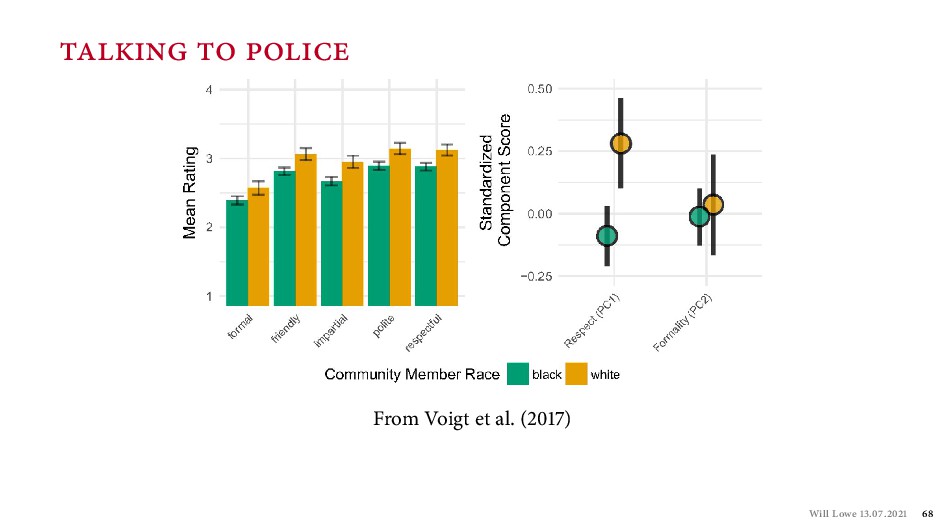
152. Riker, W. H., Calvert, R. L., Mueller, J. E., & Wilson, R. K. ( ). “ e strategy of rhetoric: Campaigning for the American constitution.” Yale University Press. Roberts, M. E., Stewart, B. M., Tingley, D., Lucas, C., Leder-Luis, J., Gadarian, S. K., Albertson, B., & Rand, D. G. ( ). “Structural Topic Models for open-ended survey responses.” American Journal of Political Science, ( ), – . Searle, J. R. ( ). “ e construction of social reality.” Free Press. Slapin, J. B., & Proksch, S.-O. ( ). “A scaling model for estimating time-series party positions from texts.” American Journal of Political Science, ( ), – . Voigt, R., Camp, N. P., Prabhakaran, V., Hamilton, W. L., Hetey, R. C., Gri ths, C. M., Jurgens, D., Jurafsky, D., & Eberhardt, J. L. ( ). “Language from police body camera footage shows racial disparities in o cer respect.” Proceedings of the National Academy of Sciences, ( ), – . Will Lowe . .
153. Zhang, H., & Maloney, L. T. ( ). “Ubiquitous log odds: A common representation of probability and frequency distortion in perception, action, and cognition.” Frontiers in Neuroscience, . Zipf, G. K. ( ). “Selected studies of the principle of relative frequency in language.” Oxford University Press. Will Lowe . .