The Release of the GEM Global Active Faults Database and Global Seismic Hazard Map

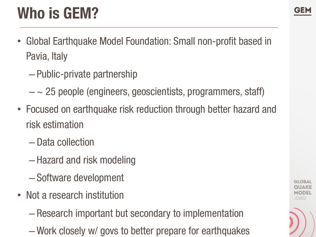
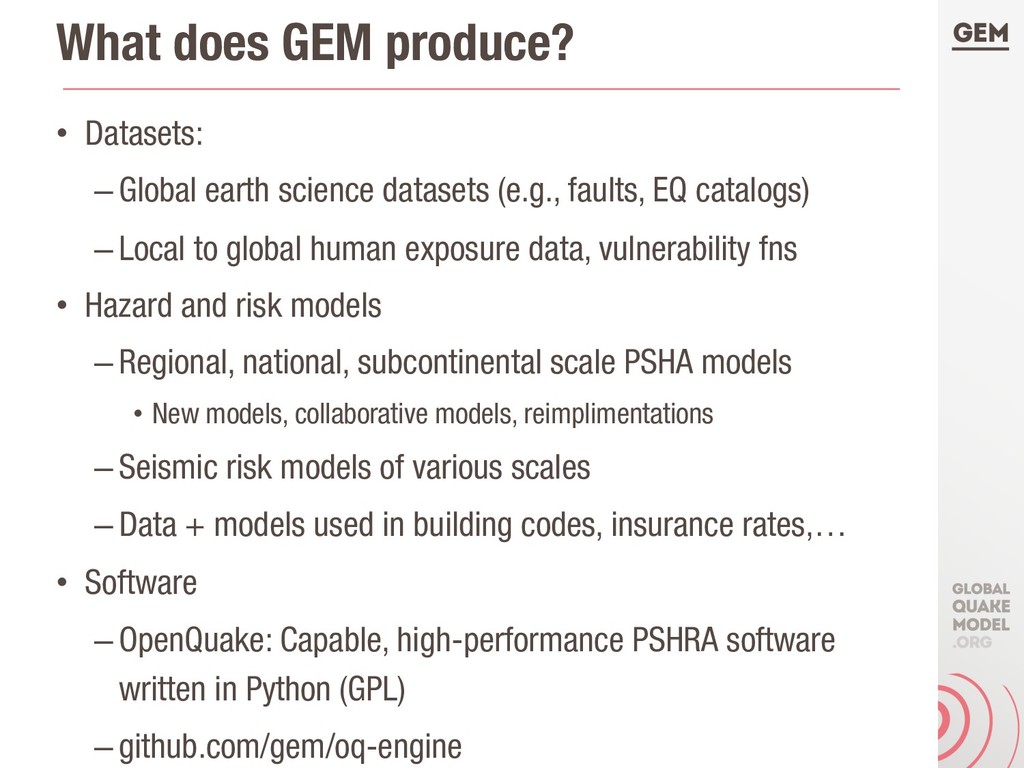
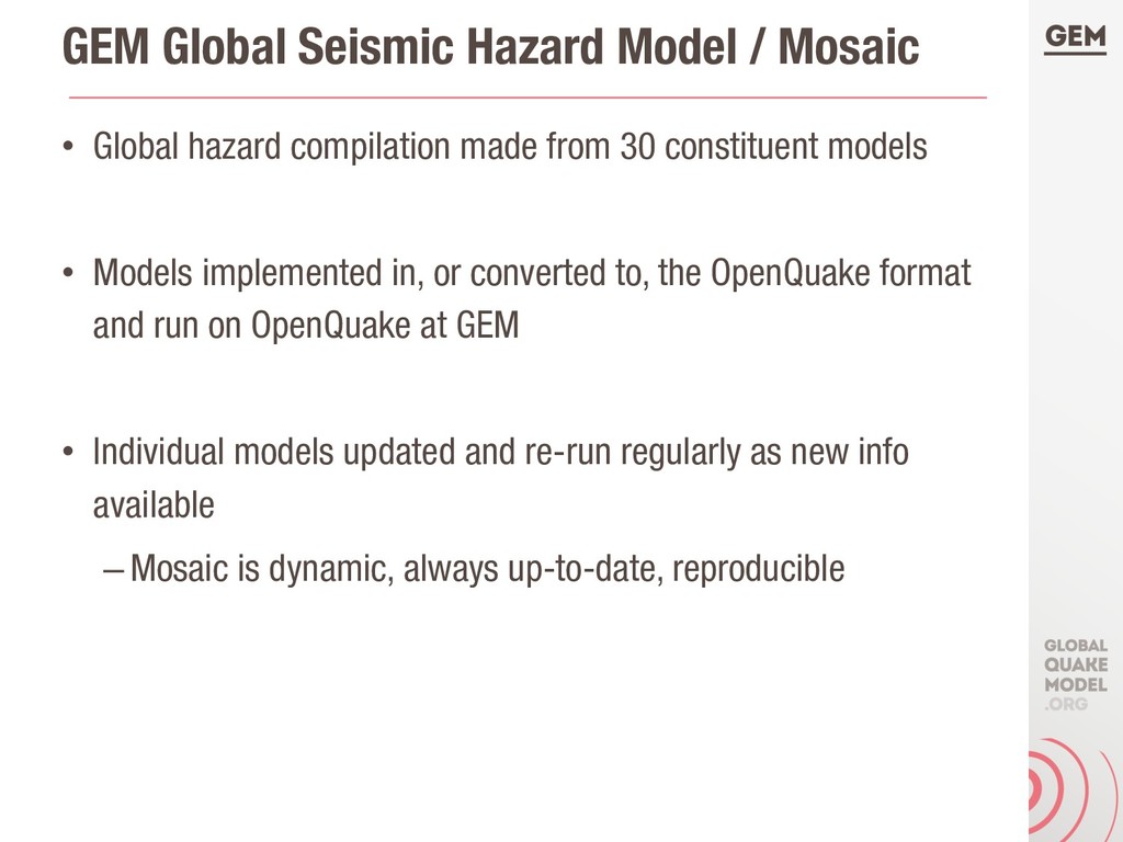
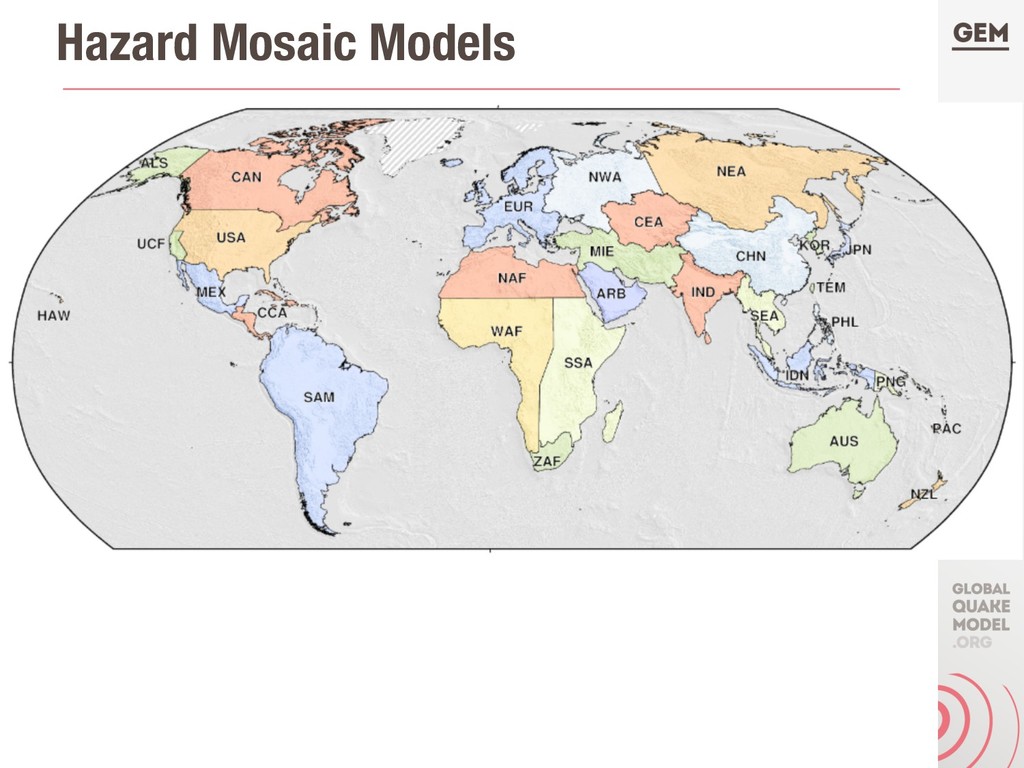
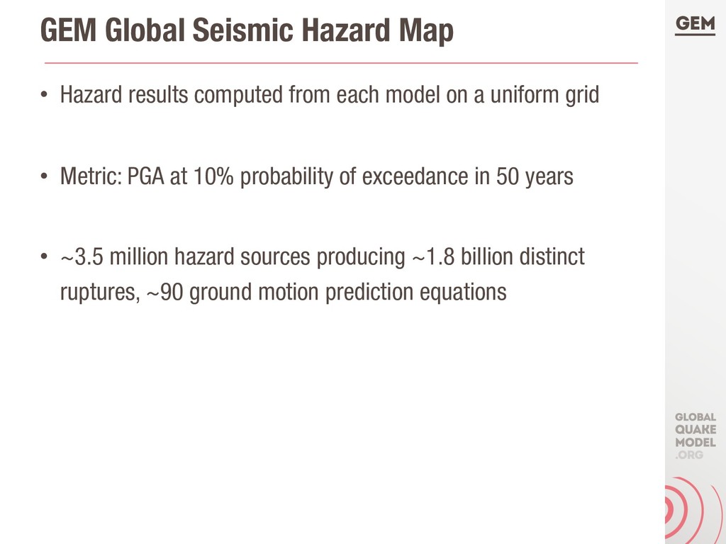
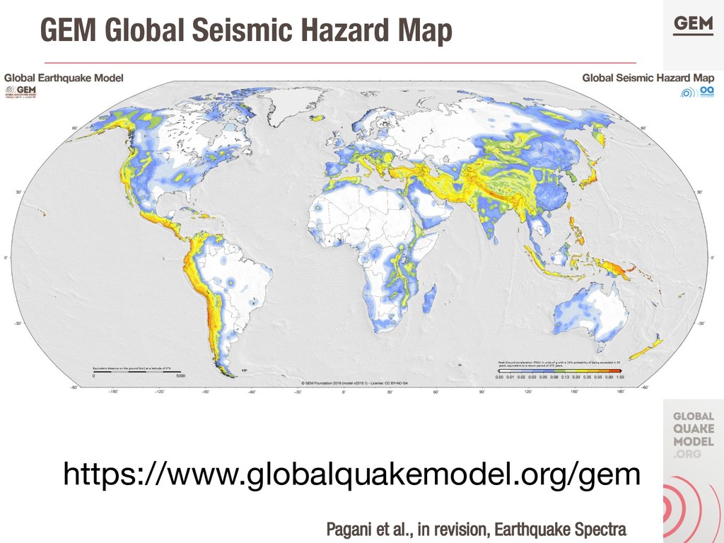
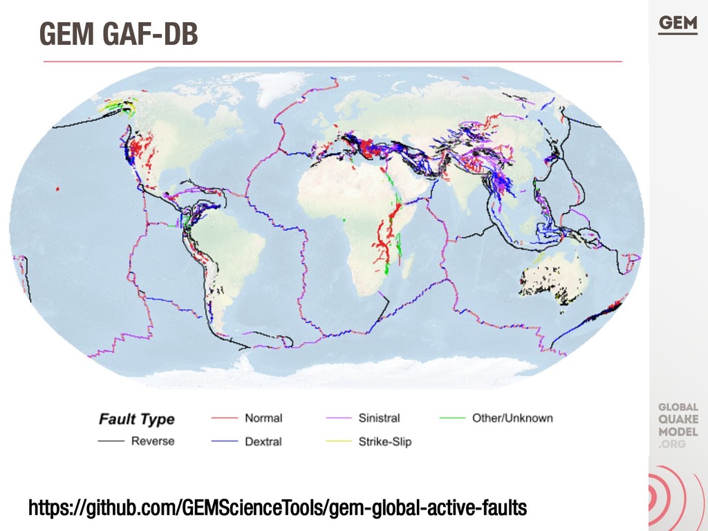
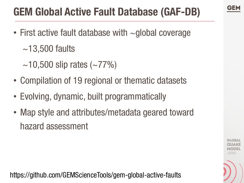
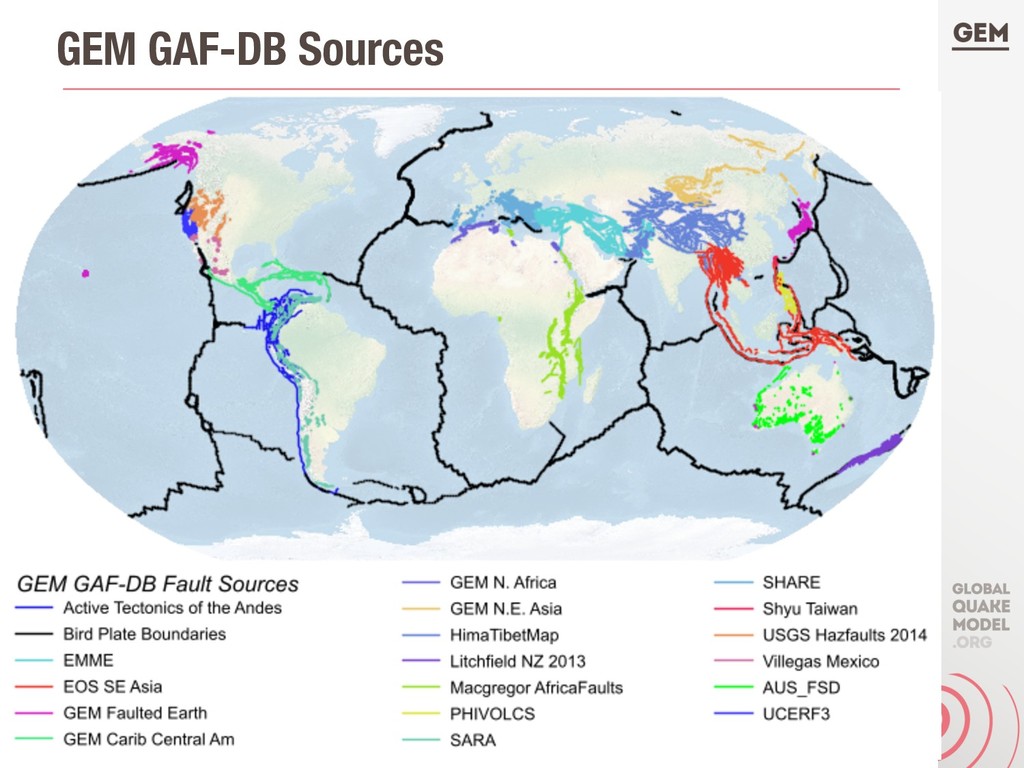
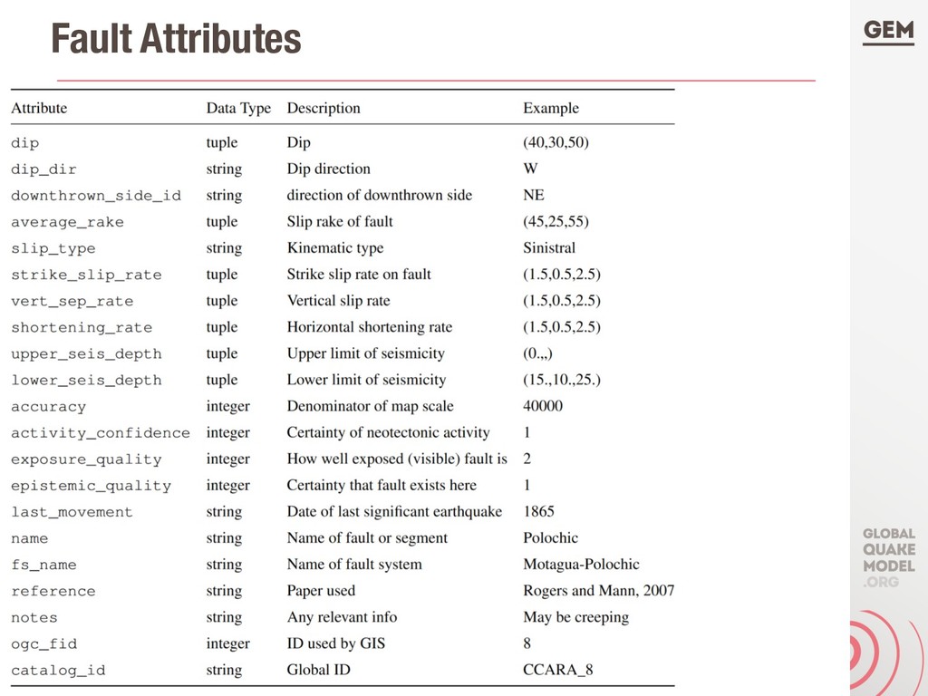
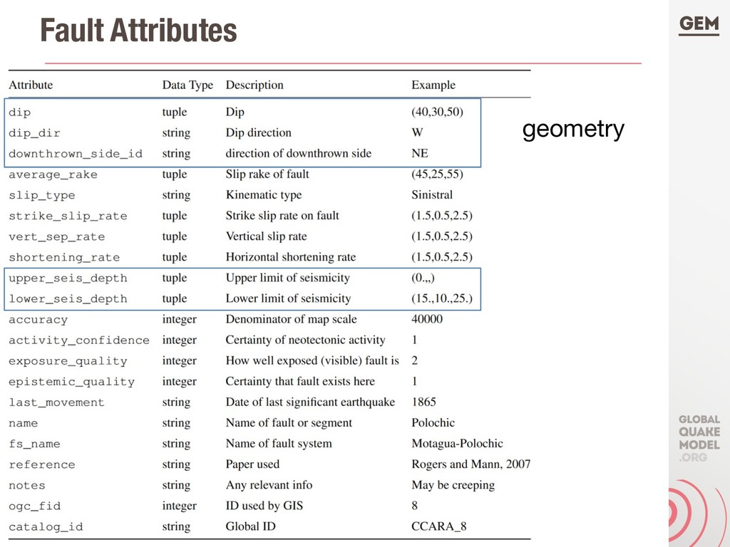
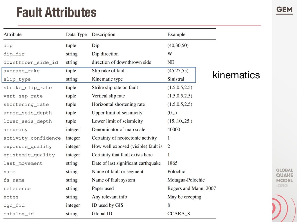
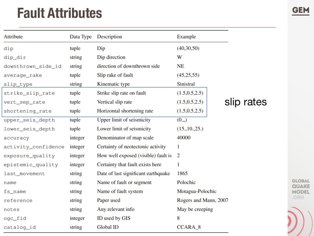
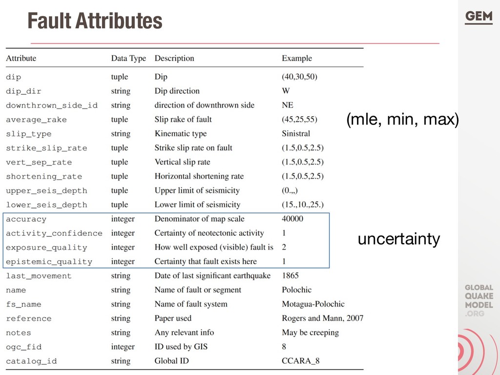
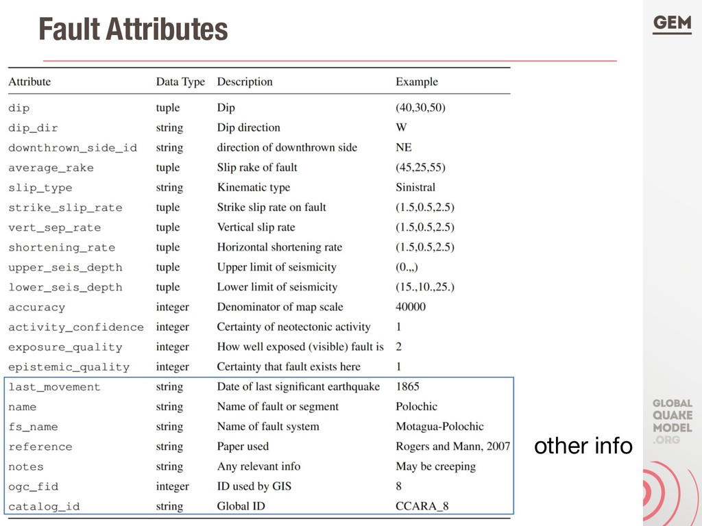
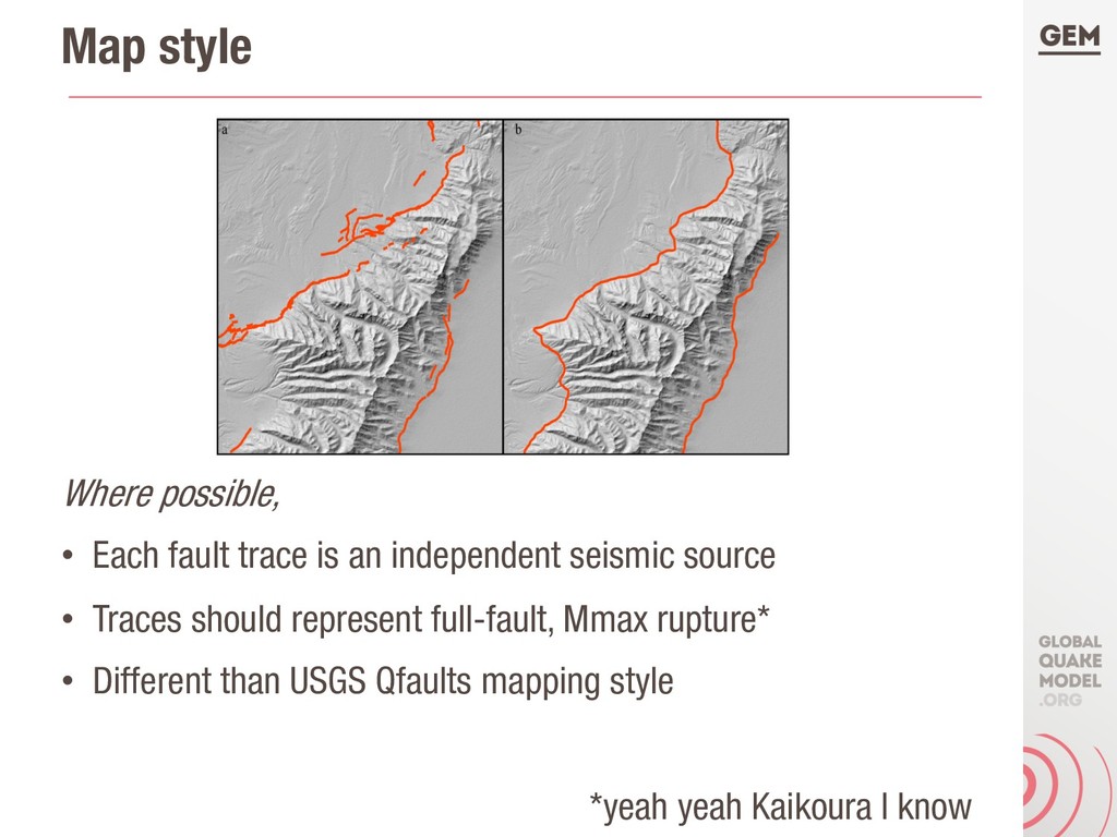
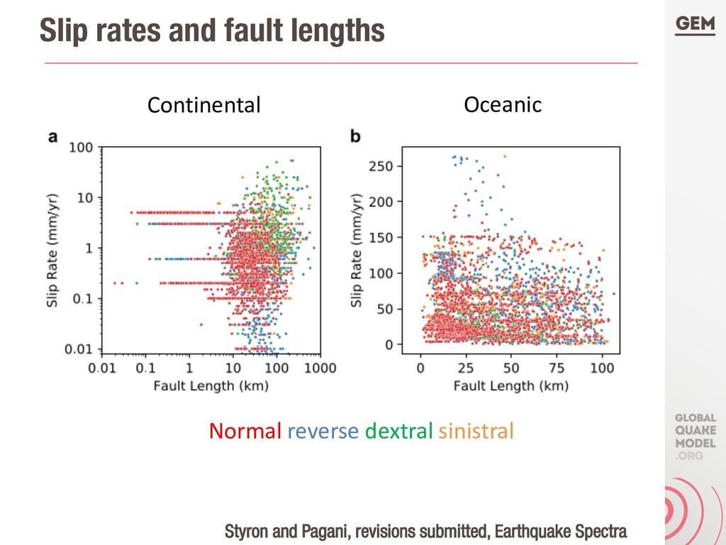
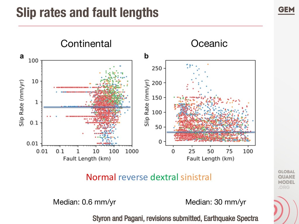
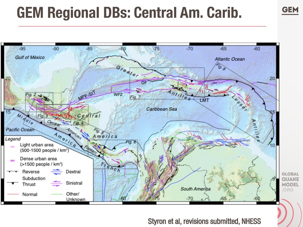
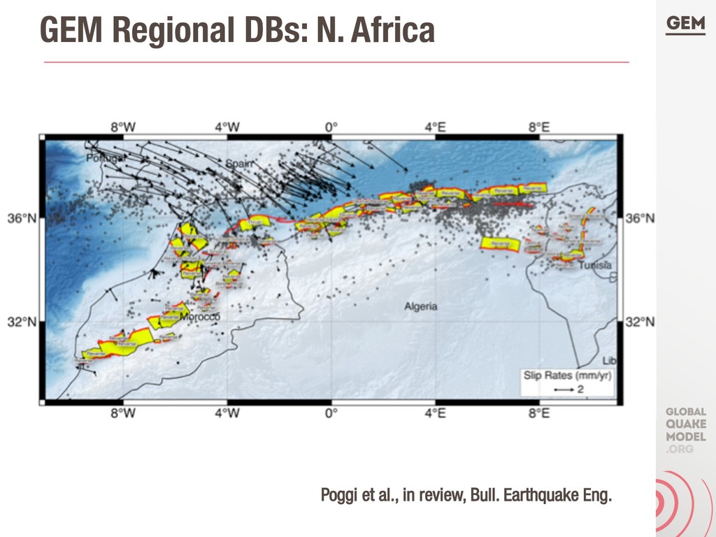
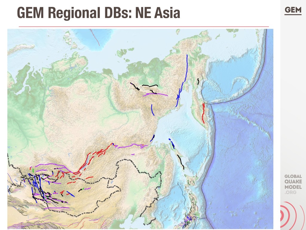
In late 2018, the Global Earthquake Model Foundation (GEM) released the initial version of several major products relating to seismic hazard and risk, including the Global Seismic Hazard Map, the Global Seismic Risk Map, and the Global Active Faults Database. Though these are intended primarily to support GEM's mission to reduce earthquake risk, they may be of use or interest to geodynamics researchers and the broader Earth science community. The GEM Global Active Faults Database (github.com/GEMScienceTools/gem-global-active-faults) is a dynamic, evolving compilation of active faults worldwide, currently containing ~14,000 fault traces. Associated metadata describe the geometry, kinematics, slip rates and other parameters relevant to seismic hazard analysis. Metadata completeness varies regionally, with ~75% of faults having some slip rate information. The GEM Global Seismic Hazard Map (globalquakemodel.org/gem) displays the geographic distribution of Peak Ground Acceleration with a 10% probability of exceedance in 50 years, and is derived from a mosaic of national or regional seismic hazard models created by a variety of organizations including the GEM Secretariat. Additional topics of collaboration or mutual beneficial research between the geodynamics and seismic hazard communities will be discussed.

Transcript

1. The Release of the GEM Global Active Faults Database and Global Seismic Hazard Map Richard Styron Global Earthquake Model Foundation richard.styron@globalquakemodel.org CIG Webinar 2019.11.14
2. Today’s talk • Intro to seismic hazard, risk, and GEM • GEM Seismic Hazard Map and Global Active Fault Database • Topics for hazard-related geophysics research
3. What is seismic hazard and risk? • ‘Hazard’ is defined as the likelihood of an event occurring –Usually ground motions (PGA, etc.) at/above some value in some time interval at some site • Hazard is the combination of earthquake occurrence and ground motion predictions • Probabilistic Seismic Hazard Analysis (PSHA) considers all ~reasonably~ possible earthquakes, with assigned probabilities, and many ground motion models (with uncertainty) to compute a probabilistic result • ‘Risk’ is the product of the consequence of the event and the hazard –Probabilistic or deterministic (scenario events)
4. Earthquake losses • ~1.6 million earthquake deaths since 1900 (Wikipedia) • $ 661 Billion USD losses 1998-2017 (UNISDR) Data from https://ourworldindata.org/natural-disasters
5. Who is GEM? • Global Earthquake Model Foundation: Small non-profit based in Pavia, Italy –Public-private partnership –~ 25 people (engineers, geoscientists, programmers, staff) • Focused on earthquake risk reduction through better hazard and risk estimation –Data collection –Hazard and risk modeling –Software development • Not a research institution –Research important but secondary to implementation –Work closely w/ govs to better prepare for earthquakes
6. What does GEM produce? • Datasets: –Global earth science datasets (e.g., faults, EQ catalogs) –Local to global human exposure data, vulnerability fns • Hazard and risk models –Regional, national, subcontinental scale PSHA models • New models, collaborative models, reimplimentations –Seismic risk models of various scales –Data + models used in building codes, insurance rates,… • Software –OpenQuake: Capable, high-performance PSHRA software written in Python (GPL) –github.com/gem/oq-engine
7. We’re hiring! • Looking for a hazard modeler (post-doc or post-MS) –Strong background in scientific programming –Solid understanding of seismology, tectonics or PSHA • Good work environment –Impactful –Great team –Fun, challenging work • Pavia is lovely • Email jobs_hazard@globalquakemodel.org
8. GEM Global Seismic Hazard Model / Mosaic • Global hazard compilation made from 30 constituent models • Models implemented in, or converted to, the OpenQuake format and run on OpenQuake at GEM • Individual models updated and re-run regularly as new info available –Mosaic is dynamic, always up-to-date, reproducible
9. Hazard Mosaic Models
10. GEM Global Seismic Hazard Map • Hazard results computed from each model on a uniform grid • Metric: PGA at 10% probability of exceedance in 50 years • ~3.5 million hazard sources producing ~1.8 billion distinct ruptures, ~90 ground motion prediction equations
11. GEM Global Seismic Hazard Map https://www.globalquakemodel.org/gem Pagani et al., in revision, Earthquake Spectra
12. GEM GAF-DB https://github.com/GEMScienceTools/gem-global-active-faults
13. GEM Global Active Fault Database (GAF-DB) • First active fault database with ~global coverage ~13,500 faults ~10,500 slip rates (~77%) • Compilation of 19 regional or thematic datasets • Evolving, dynamic, built programmatically • Map style and attributes/metadata geared toward hazard assessment https://github.com/GEMScienceTools/gem-global-active-faults
14. GEM GAF-DB Sources
15. Fault Attributes
16. Fault Attributes geometry
17. Fault Attributes kinematics
18. Fault Attributes slip rates
19. Fault Attributes uncertainty (mle, min, max)
20. Fault Attributes other info
21. Map style Where possible, • Each fault trace is an independent seismic source • Traces should represent full-fault, Mmax rupture* • Different than USGS Qfaults mapping style *yeah yeah Kaikoura I know
22. Slip rates and fault lengths Continental Oceanic Normal reverse dextral sinistral Styron and Pagani, revisions submitted, Earthquake Spectra
23. Slip rates and fault lengths Continental Oceanic Normal reverse dextral sinistral Median: 0.6 mm/yr Median: 30 mm/yr Styron and Pagani, revisions submitted, Earthquake Spectra
24. Assembly • GAF-DB assembled programmatically from constituent datasets –Each dataset is loaded, and attributes (columns) are selected and parsed/translated to GAF-DB format with custom Python functions for that dataset –Final GAF-DB catalog is assembled and then subject to some data QA checks • Assembly takes ~1 minute • Assembly performed each time constituent datasets are updated, or new databases are added, or GAF-DB schema changes • Transparent, repeatable
25. Harmonization • GAF-DB contains overlaps between different catalogs • ‘Harmonization’ process removes faults from one catalog in case of overlaps –One catalog takes priority (faults retained) –In some cases, only intersecting (crossing) faults are considered –In others, all faults removed from lower-priority catalog if they intersect convex hull around higher-priority catalog • Repeatable, automated, no modifications to data or catalogs
26. Data Formats • The GAF-DB is a vector GIS database –Fault traces are polylines • One feature (row) per fault • No multi-line types –Metadata for each fault are GIS attributes • GeoJSON format is ‘version of record’, for editing, storing, VCS –Plain-text vector GIS format • Primary webmap format, used by QGIS, Python, etc. –Conversions to GeoPackage (SQLite), ShapeFile, GMT, etc. done after assembly and harmonization
27. Updates and Version Control • GAF-DB .geojson tracked with git version control software –1 line in file per fault: easy per-fault change tracking –Updates, contributions, schema changes all recorded, undo- able –Software development best practices (merging, forking, pull requests and change reviews, etc.) work well • Dissemination through GitHub –Extremely easy to publish changes –Users always have access to latest version + all previous versions
28. GEM Regional DBs: Central Am. Carib. Styron et al, revisions submitted, NHESS
29. GEM Regional DBs: N. Africa Poggi et al., in review, Bull. Earthquake Eng.
30. GEM Regional DBs: NE Asia
31. Topics of Hazard + Geophysics interest • All of the following topics are areas of scientific debate with hazard implications • If you’re interested in working on them with hazard modelers, please email me: • richard.styron@globalquakemodel.org
32. GEM + Geodynamics: What can you do for GEM? • PSHA based on many scientific components –Framework is reasonable –Most components could use refinement • All aspects of earthquake processes have hazard and risk implications –With PSHRA implementation, can quantify human impacts –Collaboration can focus earthquake research, increase accuracy of hazard and risk models
33. GEM + Geodynamics: What can GEM do for you? • Areas for PSHA improvement are generally scientifically uncertain • Different Earth behaviors imply different physics or geology • Linkage of statistical models or simulations with physics allows for better testing of geophysical or geological hypotheses –Generate stochastic earthquake catalogs, ground motions –Test against observations • BROADER IMPACTS
34. Fault magnitude-frequency distributions • The frequency / probability of earthquakes of different magnitudes on a fault is debated, very important for PSHA –Primary candidates: Gutenberg-Richter, Characteristic • Fault MFDs + background MFD = regional GR MFD 5.0 5.5 6.0 6.5 7.0 7.5 8.0 moment magnitude M relative frequency G-R char Styron and Hetland, 2014, GRL
35. Fault magnitude-frequency distributions • Statistical analysis of paleoseismic datasets (weakly) supports characteristic-type MFDs • Statistical and observational seismology favors Gutenberg-Richter • Modeling studies generally produce characteristic-type MFDs (given most setups) –Controlling parameters? and Sis the slip rate. The average annual release of moment is given by the annual rate of earthquakes, N, times the mean moment per earthquake, M 0 =Eqk. Setting the annual accu- mulation to be equal to the annual release, gives μASˆ NMean  M 0 Eqk  : (2) The mean moment per earthquake depends on the distri- bution of earthquake magnitudes and can be approximated by   Z Truncated-Exponential Model (a) (b) Characteristic-Earthquake Model Magnitude, M Magnitude, M Window of geologic observations above threshold of surface faulting, T Mmax Mmax T T Figure 1. Alternative models of earthquake-size distribution considered in this article. The plots, which are shown schematically to have equivalent moment-release rates, are identical at the small and moderate magnitudes sampled by the historical record but are distinct within the portion of the magnitude–frequency spectrum sampled by the paleoseismic record. (a) The truncated-exponential model predicts that the frequency of earthquakes follows a continu- ous log linear relation (equation 1, typically with bˆ 1) up to some limiting maximum-magnitude earthquake (Mmax ). (b) Under the characteristic-earthquake model, earthquakes at or near Mmax occur at the expense of smaller, moderate-magnitude events. This is re- Figure 2. Hayward fault (California) example of the discrep- ancy in rates of small-magnitude earthquakes (from a zone  5 km on either side of the fault) if moment rate on the fault is balanced and the truncated-exponential model is used with a maxi- mum magnitude based on fault dimension (Mmax 7.05, blue curve). This discrepancy can be removed by using a larger Mmax (here 8.25, orange curve) or by using the Youngs and Coppersmith (1985) char- acteristic-earthquake model (with Mchar6:8  0:25, green curve). Adapted from Geomatrix Consultants (1993). 652 S. Hecker, N. A. Abrahamson, and K. E. Wooddell Geophysical Research Letters 10.1029/2019GL083628 Figure 3. (a) Distribution of rupture lengths for simulations with a∕b = 0.75 showing characteristic distribution at Hecker et al., 2013, BSSA; Cattania, 2019, GRL
36. A Brownian Model for Recurrent Earthquakes Time Probability Density 0.0 0.5 1.0 1.5 2.0 2.5 3.0 0.0 0.2 0.4 0.6 0.8 1.0 Model BPT Lognormal Gamma Weibull Exponential Cumulative Distribution 0.0 0.5 1 0.0 0.2 0.4 0.6 0.8 1.0 a b Figure 1. Probability density (a) and cumulative distribution ( ponential (Poisson), BPT, log–normal, gamma, and Weibull mode have mean 1 and standard deviation 0.5 (except the exponential di timum model for a variety of probability distributions. His results strongly suggest that empirical analysis can discrim- inate against the exponential model, but hope for any elu- cidation beyond that level is futile with presently available data. The Brownian Relaxation Oscillator The analysis of series of events, in particular, failure- time data, has wide application across the sciences (Cox and Lewis, 1966; Kalbfleisch and Prentice, 1980). Throughout the literature, the exponential, lognormal, Weibull, and gamma distributions have been widely used as models for stationary-point processes. As discussed in the preceeding section, empirical fitting of these models to data may capture the main features of interest, but they give no insight into the process. Alternatively, models can be constructed on more theoretical grounds that achieve the same measure of The relaxation which the obvious an obvious answer. cumulative elastic (1910), but it could variables, like cum stress. It might also the unknown locati sion of each cycle, this juncture, the lo of rupture potential Let Y0 (t) denot scale where the pos is xf ס x0 ם d, d and Y0 (0) ס x0 . R occur at times tk D ס “ ”, read “is defin D ס side of an equation Exponential ␯eמnut → ␯מ1 1 hϽ 1 f→ ϱ Gamma h hמ1 מvt m t e C(h) hמ1 hϾ 1 F→ 0 hϽ 1 f ϱ 0 Weibull h hמ1 h h hm t exp(מm t ) hϾ 1 F 0 ϱ Lognormal מ1 2 (log tמl) 2prt exp מ Ί ΂ ΃ ΂ ΃ 2 2r Ff 0 0 Columns are as follows: 1, name of parametric family (and indication, as necessary, of parameter range restriction for following columns); 2, parametrized probability density function; 3, shape of failure-rate function: F ס increasing, f ס decreasing, → ס constant; combination of symbols indicates changing behavior with time, e.g., the BPT failure increases for some time, then decreases, and flattens out to a constant asymptotic level; 4, failure rate at t ס 0; 5, ratio of mean and quasi-stationary mean recurrence interval. Time Hazard Rate 0.0 0.5 1.0 1.5 2.0 2.5 3.0 0 1 2 3 4 5 6 Model BPT Lognormal Gamma Weibull Exponential and increase to a finite asymptotic level that is always smaller than the mean recurrence rate. Hence, these distri- butions cannot produce behavior equivalent to the signal- dominated regime in the Brownian passage-time family. Figure 5 shows plots of the hazard-rate functions for the five distributions under discussion (see also Fig. 1 for the corresponding probability density functions [pdfs]). The pa- rameters for each distribution are set so that the mean re- currence time is equal to 1. For all but the exponential, which has only one adjustable parameter, the aperiodicity is equal to 1/2. Although ␣ ס 1/2 is selected here for illustration, Ellsworth et al. (1999) proposed this as a generic aperiodic- ity based on 37 recurrent earthquake sequences, מ0.7 Յ M Յ 9.2. There are several noteworthy comparisons to be made of the probability densities as well (Fig. 1). The lognormal and BPT functions put least weight in the left tail, near t ס 0. For these two distributions, the density and hazard rate are essentially zero for about the first 25% of the mean re- currence interval. This behavior seems desirable in light of the strain-budget interpretation of elastic rebound and con- trasts with the Weibull and gamma functions, which increase relatively steeply from zero at t ס 0. All density functions are unimodal, with mode left of the mean. The lognormal is Earthquake recurrence/ time dependence • PSHA models are typically time- independent (Poisson) –Hazard doesn’t depend on time since last event • Quasi-periodic earthquakes on large faults are thoroughly embedded in earth science mindset • Statistical seismologists often favor Poisson/time-independent recurrence Matthews et al., 2002, BSSA
37. Earthquake clustering • Abundant observational evidence for earthquake clustering within fault network (and maybe across the globe) • Generally assumed to be from fault interaction (stress/strain triggering) • Changing boundary/loading conditions could also be responsible -14 -10 -6 -2 0 2 Thousand Year (C.E.) Styron and Sherrod, 2016, AGU fall meeting
38. Fault interaction • If faults interact, modeling is more complicated –Independent probabilities of rupture calculated independently –Many interacting faults mean massively dependent probabilities, lots of state –Markov or probabilistic graphical model techniques? • What are the different modes of fault interaction? • What are the resulting patterns of seismicity? • What do they imply about lithospheric properties or behavior?
39. Slip rates • How much do slip rates change with time, and why? • Do geodetic, paleoseismological, neotectonics and various bedrock geologic techniques measure the same processes? –No. But does how much it matter? –What best predicts near-future earthquake occurrence? Geophysical Research Letters 10.1002/2017GL075048 Zinke et al., 2017, GRL
40. Slip rates • How are regional deformation budgets distributed among faults? • Can slip rates ‘trade off’ on faults in a network? • Do areas of significant aseismic strain rate exist? Figure 1. (a) Shaded‐relief topography of the Tien Shan showing GPS velocity field relative to Eurasia (Zubovich et al., 2010). (b, c) GPS velocities relative to Eurasia and swath topography projected onto profile lines drawn orthogonal to 10.1029/2018TC005433 Tectonics Campbell et al., 2019, Tectonics
41. Seismicity in slow-strain rate regions • Very hard to estimate locations and rates of earthquakes in low-strain rate regions • Cold crust -> high ground shaking -> PSHA bullseyes around past events Pagani et al., in revision, Earthquake Spectra
42. Seismicity in slow-strain rate regions • How different will patterns of seismicity be over the next 100 years compared to the past 100 years? • Is seismicity caused by tectonic stress/strain or by other processes (post-glacial rebound, thermal stresses…)? • Limited to pre-existing fault zones?
43. Ground motions • Ground motion prediction equations have huge uncertainties, variability • How to model seismic attenuation across tectonic boundaries? • How to deal with variable site conditions within a model? • Machine learning models? Robin Gee, personal communication
44. How are faults loaded? • Fault loading through creep at depth means earthquakes are consequence of fault slip at depth • Fault loading by elastic crustal stresses means earthquakes and fault slip are consequences of farther-field stress Alternatively, the earthquake recurrence interval g can be adjusted by the clock change as g = g 0 + T 0. [5] The rate that faults are stressed by tectonic loading is an essential parameter for assessing hazard when earthquake nteractions have occurred. Confidence in stress change calculations has grown through repeated correlation with seismicity rate changes [e.g., Harris, 1998, and references herein]. Less is understood about tectonic stressing of ndividual faults. This study builds on previous finite element modeling of California and the San Francisco Bay region Ben-Zion et al., 1993; Furlong and Verdonck, 1994; Bird and Kong, 1994; Reches et al., 1994; Wang et al., 1995; Wang and Cai, 1997; Kenner and Segall, 1999; Geist and Andrews, 2000] and is conducted for the purpose of determining ectonic stressing rates for seismic hazard application. PARSONS: POST-1906 STRESS RECOVERY OF SAN ANDREAS SYSTEM ESE 3 - 3 • Different loading models predict different modes of fault interaction and likelihood of off-fault seismicity Parsons, 2002, JGR
45. Questions? Comments? • Thanks for watching/reading! • Please contact me: –richard.styron@globalquakemodel.org