PMI-ACP PMI-RMP CSM LSSGB Project Management Professional Agile Cer4fied Prac44oner Risk Management Professional Cer4fied Scrum Master Lean Six Sigma Green Belt LSSBB SSMBB ITIL Lean Six Sigma Black Belt Six Sigma Master Black Belt Informa4on Technology Infrastructure Library Agile PM Dynamic System Development Methodology Atern Name: Bharani Kumar Educa+on: IIT Hyderabad Indian School of Business Professional cer+fica+ons:
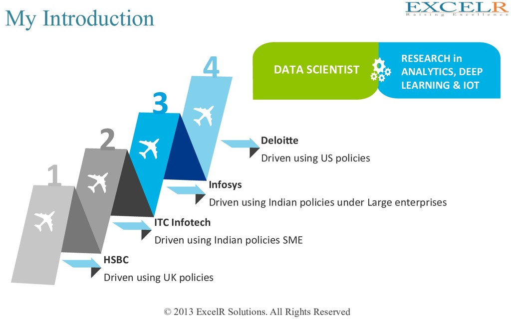
Driven using UK policies ITC Infotech Driven using Indian policies SME Infosys Driven using Indian policies under Large enterprises DeloiHe Driven using US policies 1 2 3 4 RESEARCH in ANALYTICS, DEEP LEARNING & IOT DATA SCIENTIST
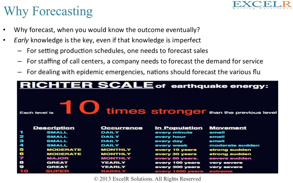
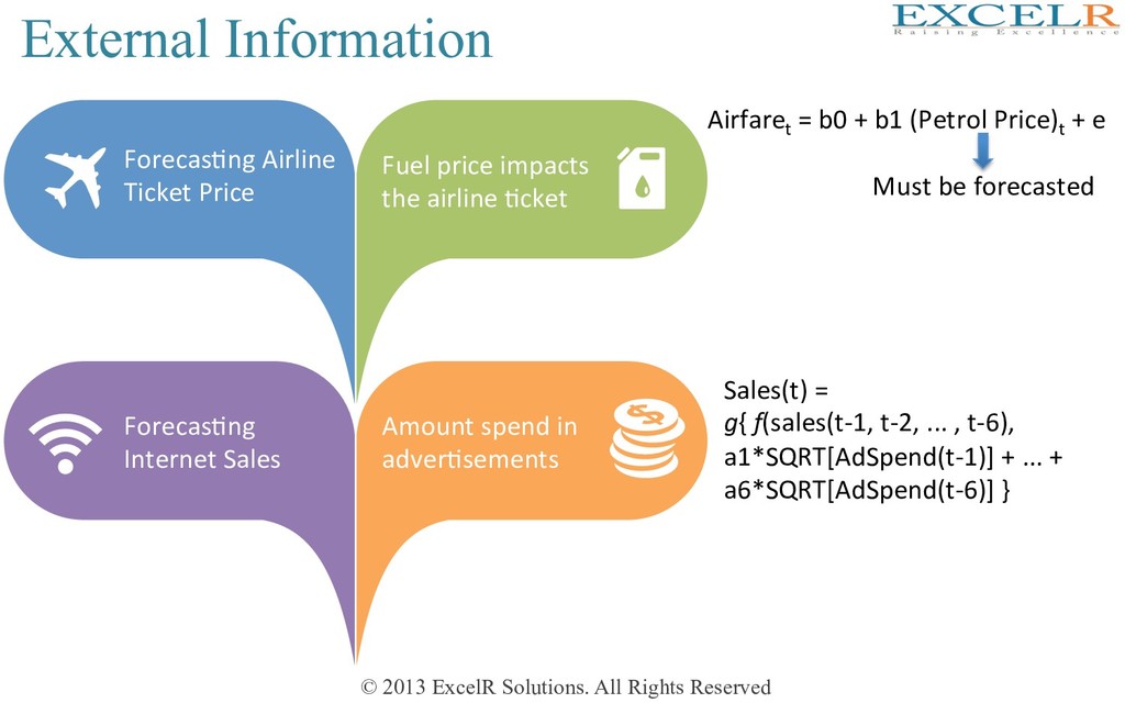
Why forecast, when you would know the outcome eventually? • Early knowledge is the key, even if that knowledge is imperfect – For seQng producHon schedules, one needs to forecast sales – For staffing of call centers, a company needs to forecast the demand for service – For dealing with epidemic emergencies, naHons should forecast the various flu
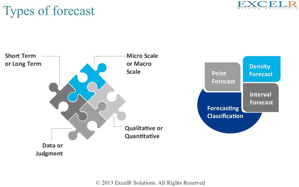
Micro Scale or Macro Scale Qualita4ve or Quan4ta4ve Short Term or Long Term Data or Judgment Forecas4ng Classifica4on Point Forecast Density Forecast Interval Forecast
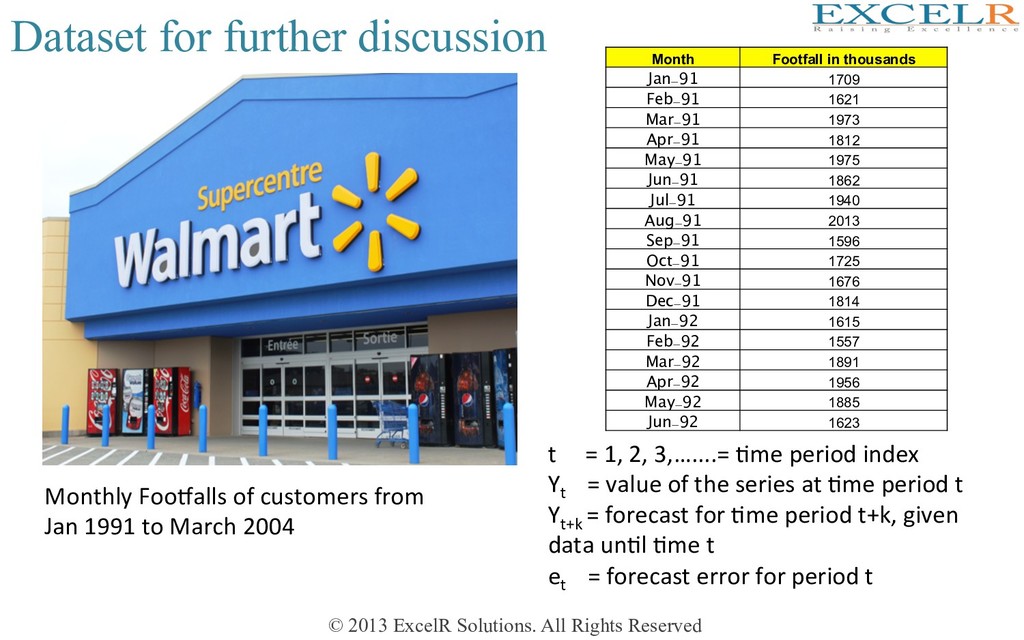
discussion Monthly FooWalls of customers from Jan 1991 to March 2004 t = 1, 2, 3,…....= Hme period index Yt = value of the series at Hme period t Yt+k = forecast for Hme period t+k, given data unHl Hme t et = forecast error for period t Month Footfall in thousands Jan-91 1709 Feb-91 1621 Mar-91 1973 Apr-91 1812 May-91 1975 Jun-91 1862 Jul-91 1940 Aug-91 2013 Sep-91 1596 Oct-91 1725 Nov-91 1676 Dec-91 1814 Jan-92 1615 Feb-92 1557 Mar-92 1891 Apr-92 1956 May-92 1885 Jun-92 1623
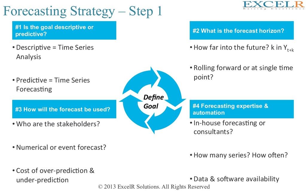
Step 1 • DescripHve = Time Series Analysis • PredicHve = Time Series ForecasHng • How far into the future? k in Yt+k • Rolling forward or at single Hme point? #1 Is the goal descriptive or predictive? #2 What is the forecast horizon? • Who are the stakeholders? • Numerical or event forecast? • Cost of over-predicHon & under-predicHon • In-house forecasHng or consultants? • How many series? How ofen? • Data & sofware availability #3 How will the forecast be used? #4 Forecasting expertise & automation Define Goal
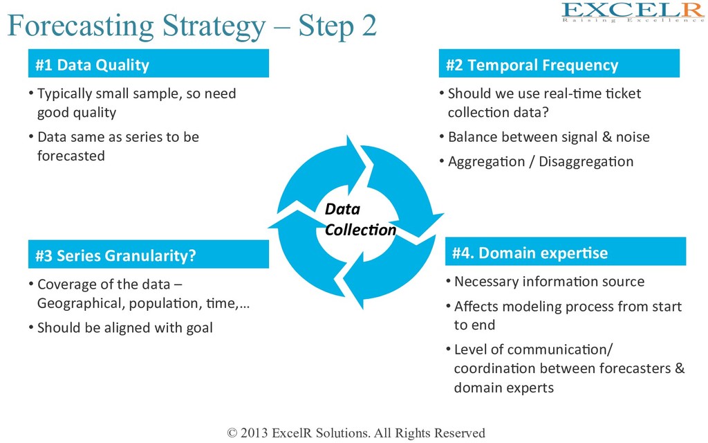
Step 2 • Typically small sample, so need good quality • Data same as series to be forecasted • Should we use real-Hme Hcket collecHon data? • Balance between signal & noise • AggregaHon / DisaggregaHon #1 Data Quality #2 Temporal Frequency • Coverage of the data – Geographical, populaHon, Hme,… • Should be aligned with goal • Necessary informaHon source • Affects modeling process from start to end • Level of communicaHon/ coordinaHon between forecasters & domain experts #3 Series Granularity? #4. Domain exper4se Data Collec-on
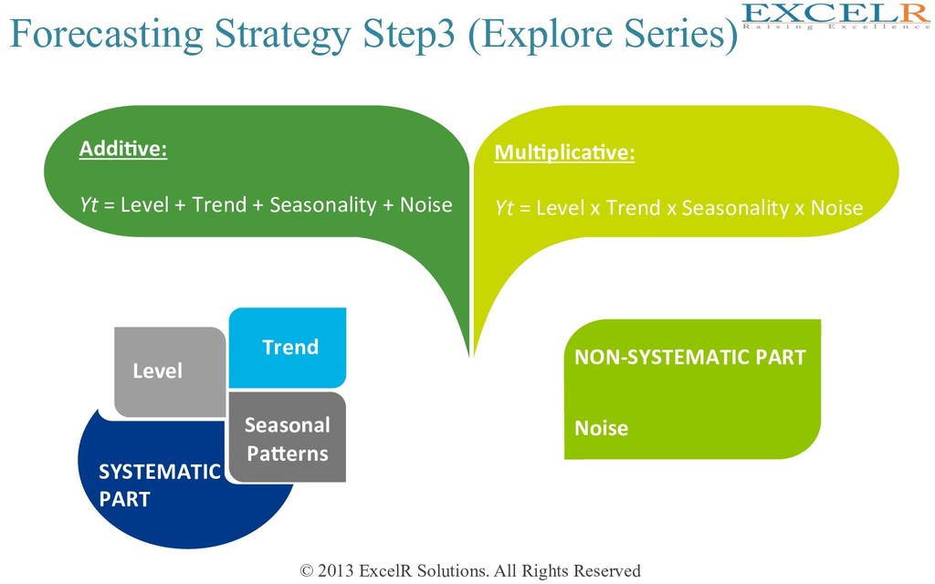
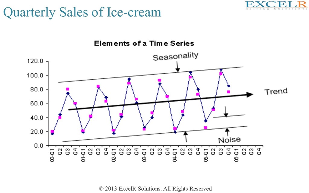
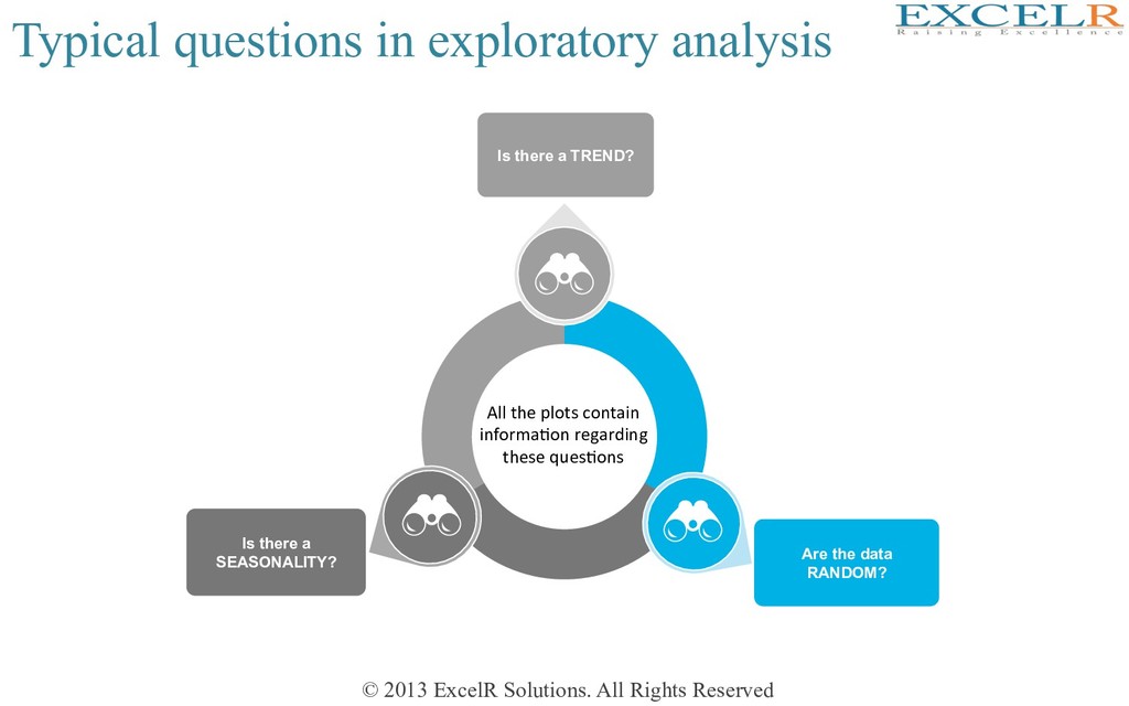
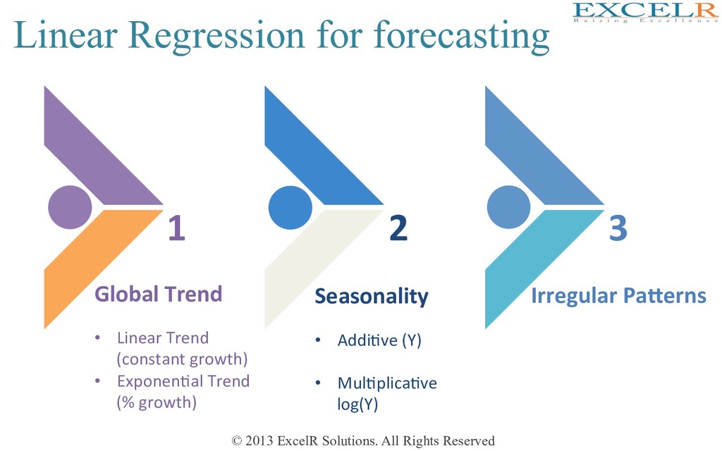
(Explore Series) Seasonal PaHerns SYSTEMATIC PART Level Trend Season al PaHern s NON-SYSTEMATIC PART Noise Addi4ve: Yt = Level + Trend + Seasonality + Noise Mul4plica4ve: Yt = Level x Trend x Seasonality x Noise
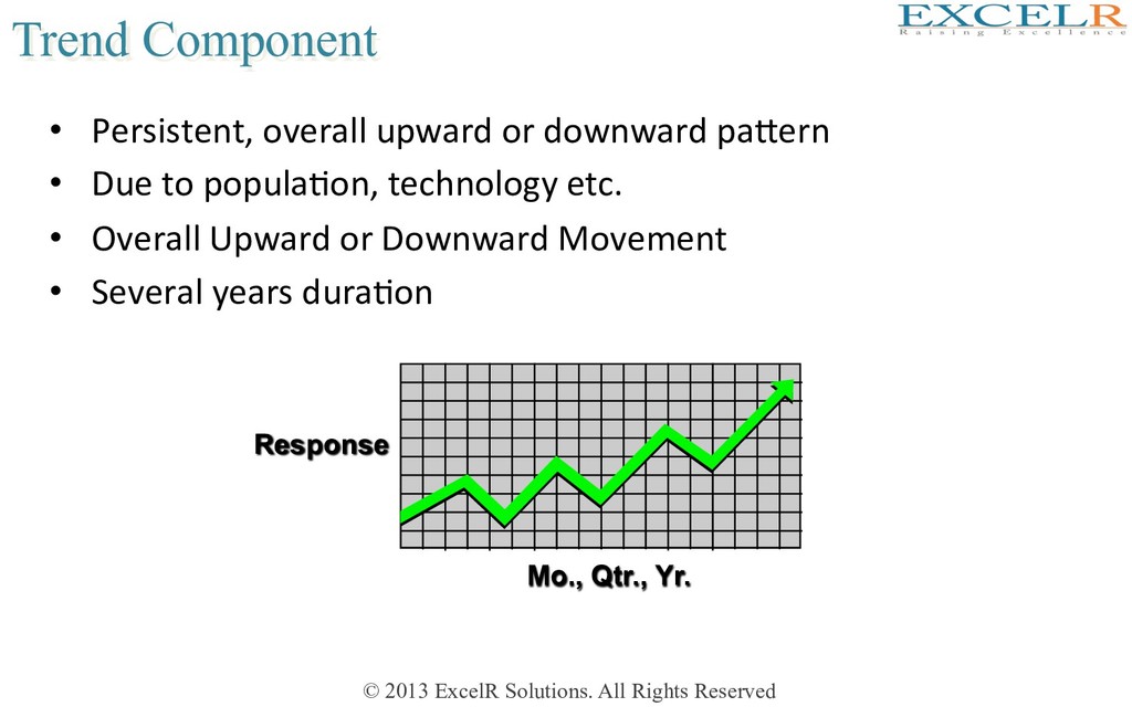
Persistent, overall upward or downward paKern • Due to populaHon, technology etc. • Overall Upward or Downward Movement • Several years duraHon Mo., Qtr., Yr. Response
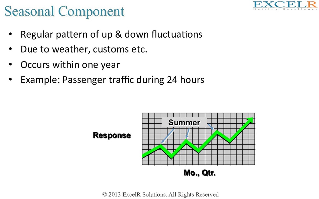
Regular paKern of up & down fluctuaHons • Due to weather, customs etc. • Occurs within one year • Example: Passenger traffic during 24 hours Mo., Qtr. Response Summer
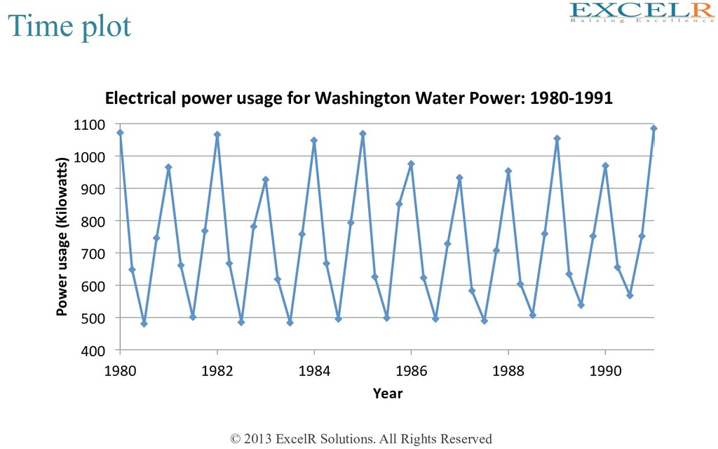
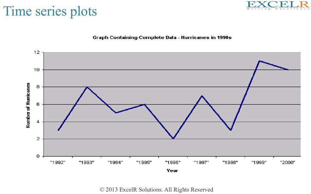
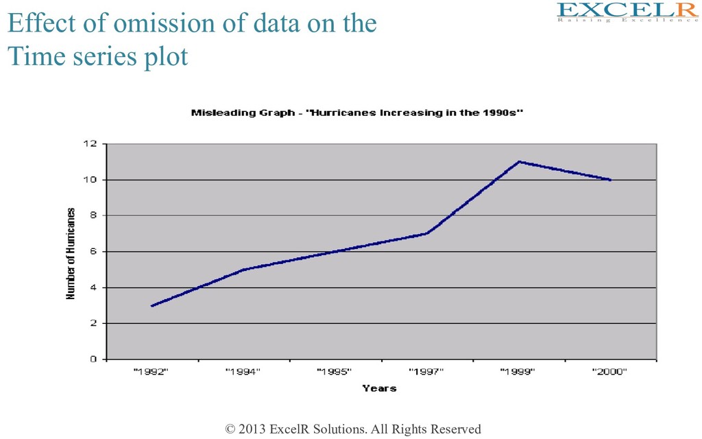
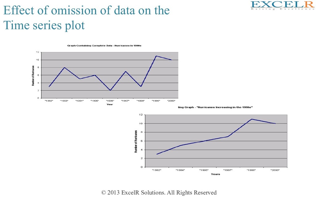
Plots a variable against Hme index • Appropriate for visualizing serially collected data (Hme series) • Brings out many useful aspects of the structure of the data • Example: Electrical usage for Washington Water Power (Quarterly data from 1980 to 1991)
is a cyclic trend • Maximum demand in first quarter; minimum in third quarter • There may also be a slowly increasing trend (to be examined) • Any reasonable forecast should have cyclic fluctuaHons • Trend (if any) need to be uHlized for forecasHng • Forecast would not be exact – there would be some error
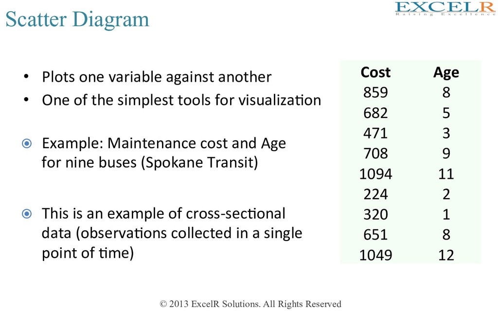
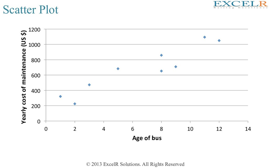
Plots one variable against another • One of the simplest tools for visualizaHon Cost Age 859 8 682 5 471 3 708 9 1094 11 224 2 320 1 651 8 1049 12 Example: Maintenance cost and Age for nine buses (Spokane Transit) This is an example of cross-secHonal data (observaHons collected in a single point of Hme)
buses have higher cost of maintenance • There is some variaHon (case to case) • The rise in cost is about $ 80 per year of age • It may be possible to use ‘age’ to forecast maintenance cost • Forecast would not be a ‘certain’ predicHon – there would be some error
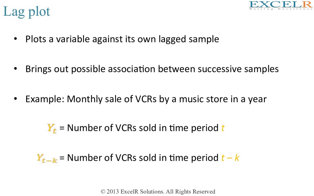
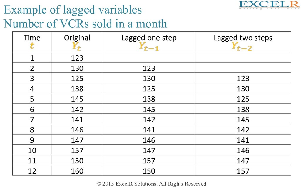
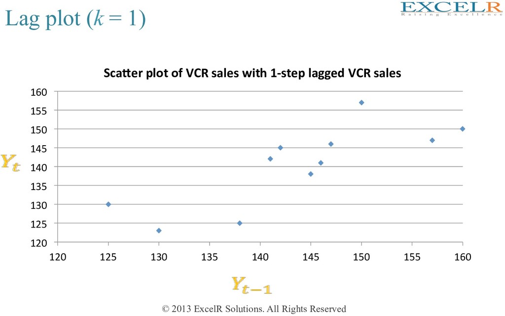
Plots a variable against its own lagged sample • Brings out possible associaHon between successive samples • Example: Monthly sale of VCRs by a music store in a year = Number of VCRs sold in Hme period t = Number of VCRs sold in Hme period t – k
is a reasonable degree of associaHon between the original variable and the lagged one • Value of lagged variable is known beforehand, so it is useful for predicHon • AssociaHon between original and lagged variable may be quan+fied through a correlaHon
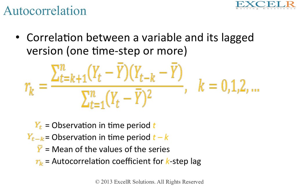
between a variable and its lagged version (one Hme-step or more) = ObservaHon in Hme period t = ObservaHon in Hme period t – k = Mean of the values of the series = AutocorrelaHon coefficient for k-step lag
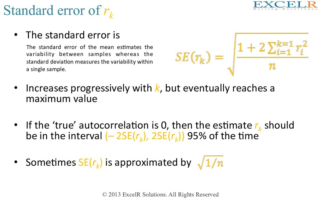
rk • The standard error is • Increases progressively with k, but eventually reaches a maximum value • If the ‘true’ autocorrelaHon is 0, then the esHmate rk should be in the interval (– 2SE(rk ), 2SE(rk )) 95% of the Hme • SomeHmes SE(rk ) is approximated by The standard error of the mean esHmates the variability between samples whereas the standard deviaHon measures the variability within a single sample.
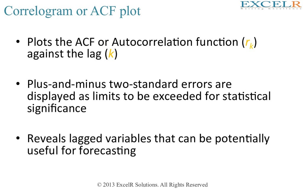
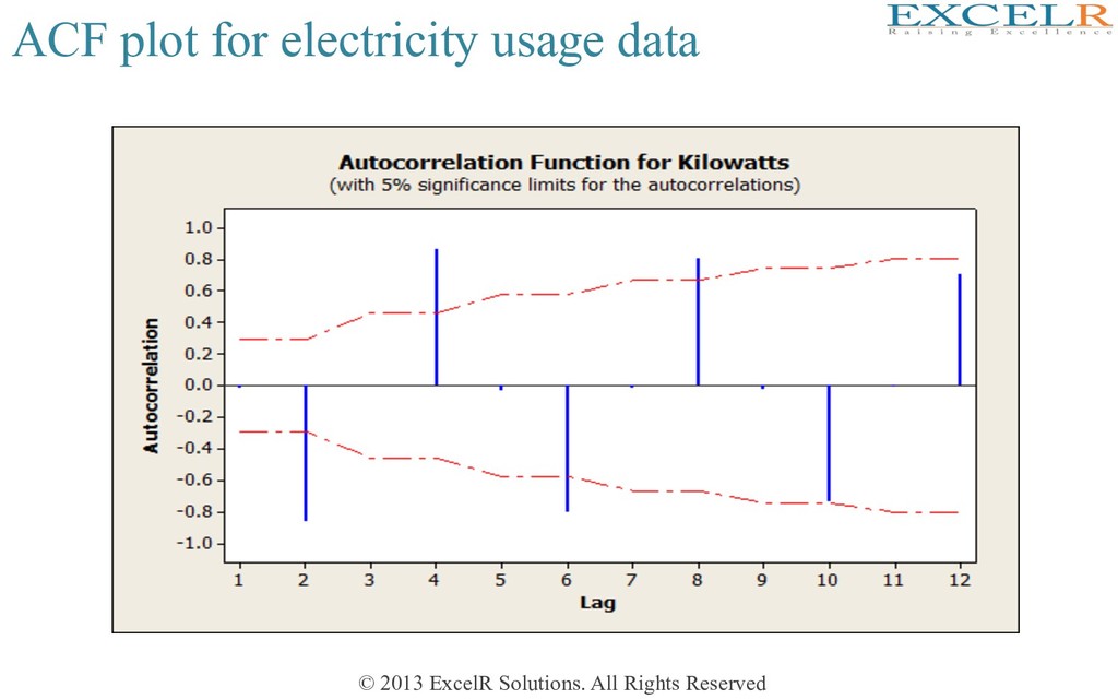
plot • Plots the ACF or AutocorrelaHon funcHon (rk ) against the lag (k) • Plus-and-minus two-standard errors are displayed as limits to be exceeded for staHsHcal significance • Reveals lagged variables that can be potenHally useful for forecasHng
alternate sample is large, many of them staHsHcally significant also • ACFs at lags 4, 8, 12, etc are posiHve • ACF at lags 2,6,10 etc are negaHve • All these pick up the seasonal aspect of the data • The data may be re-examined afer ‘removing’ seasonality
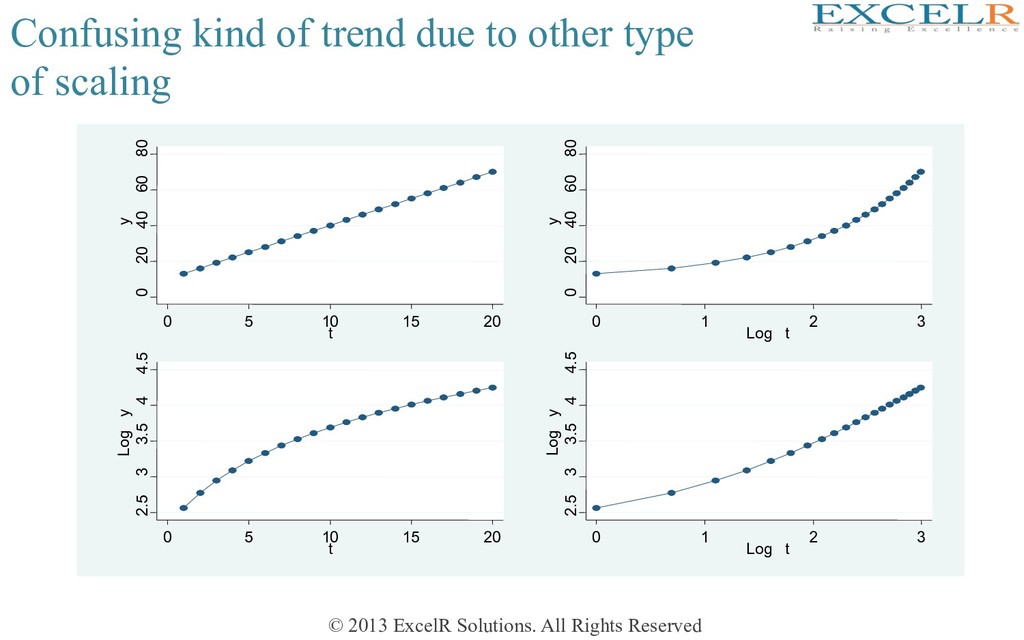
trend due to other type of scaling 0 20 40 60 80 y 0 5 10 15 20 t 0 20 40 60 80 y 0 1 2 3 Log t 2.5 3 3.5 4 4.5 Log y 0 5 10 15 20 t 2.5 3 3.5 4 4.5 Log y 0 1 2 3 Log t
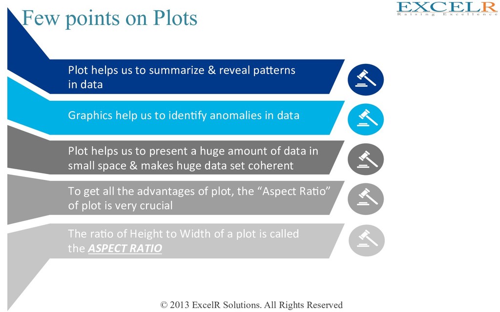
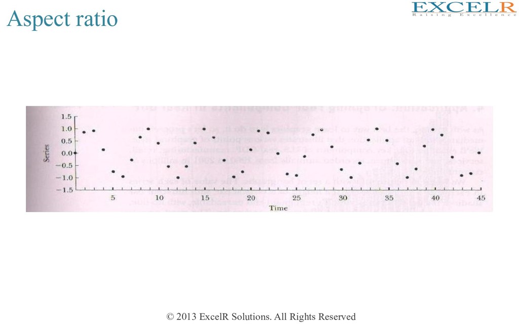
Plots Plot helps us to summarize & reveal paKerns in data Graphics help us to idenHfy anomalies in data Plot helps us to present a huge amount of data in small space & makes huge data set coherent To get all the advantages of plot, the “Aspect RaHo” of plot is very crucial The raHo of Height to Width of a plot is called the ASPECT RATIO
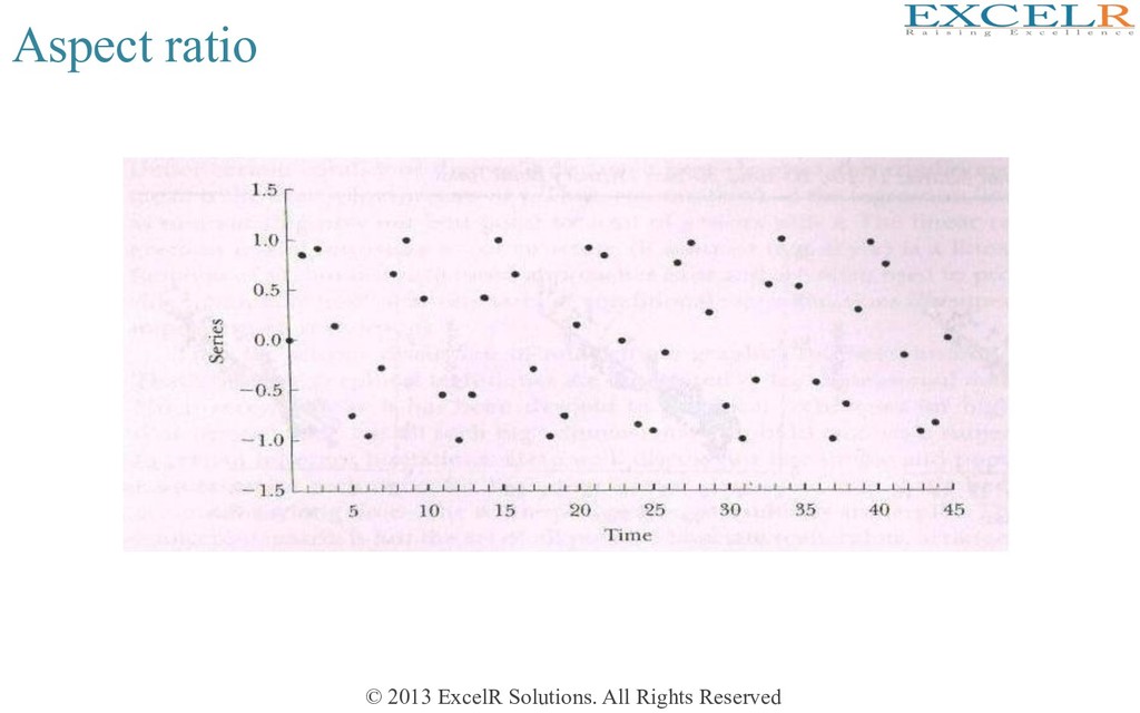
Generally aspect raHo should be around 0.618 • However, for long Hme series data aspect raHo should be around 0.25. To understand the impact of aspect raHo see the two plots in the next two slides
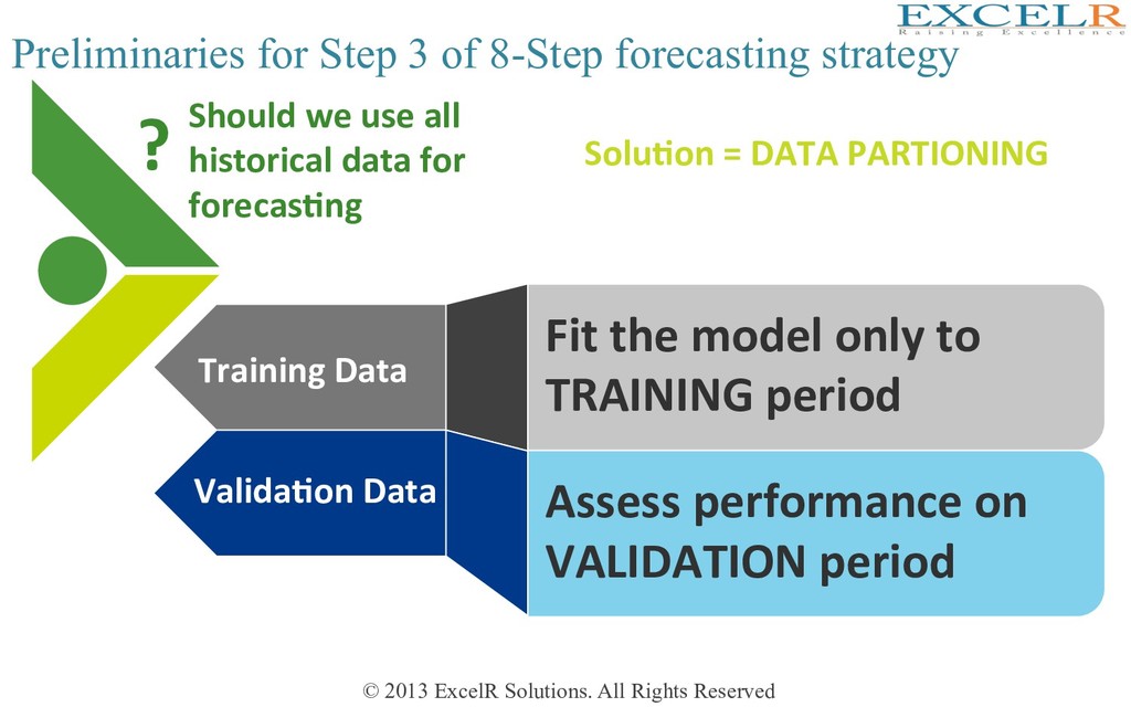
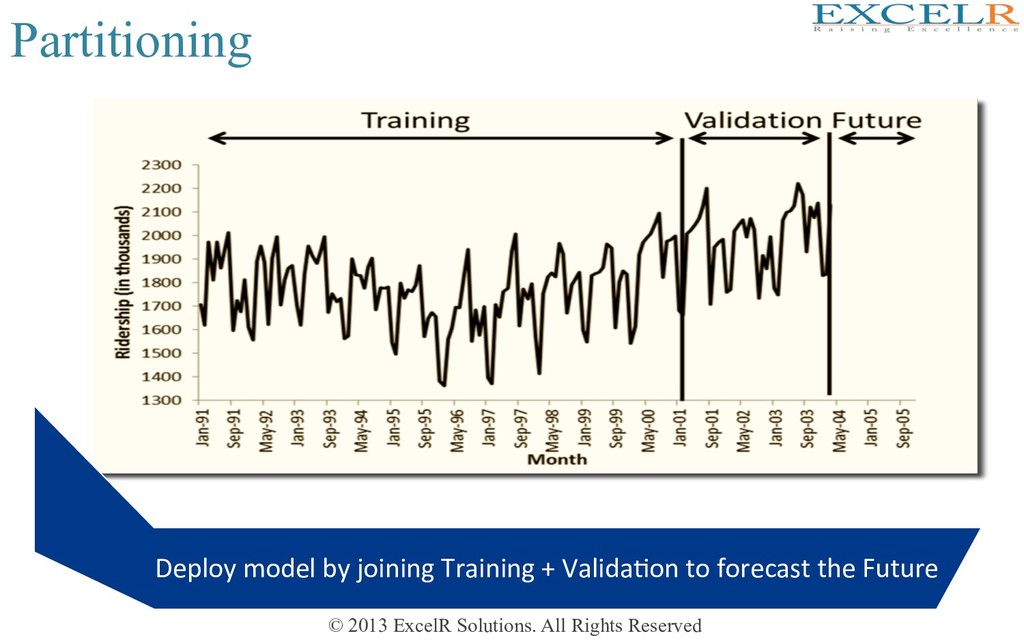
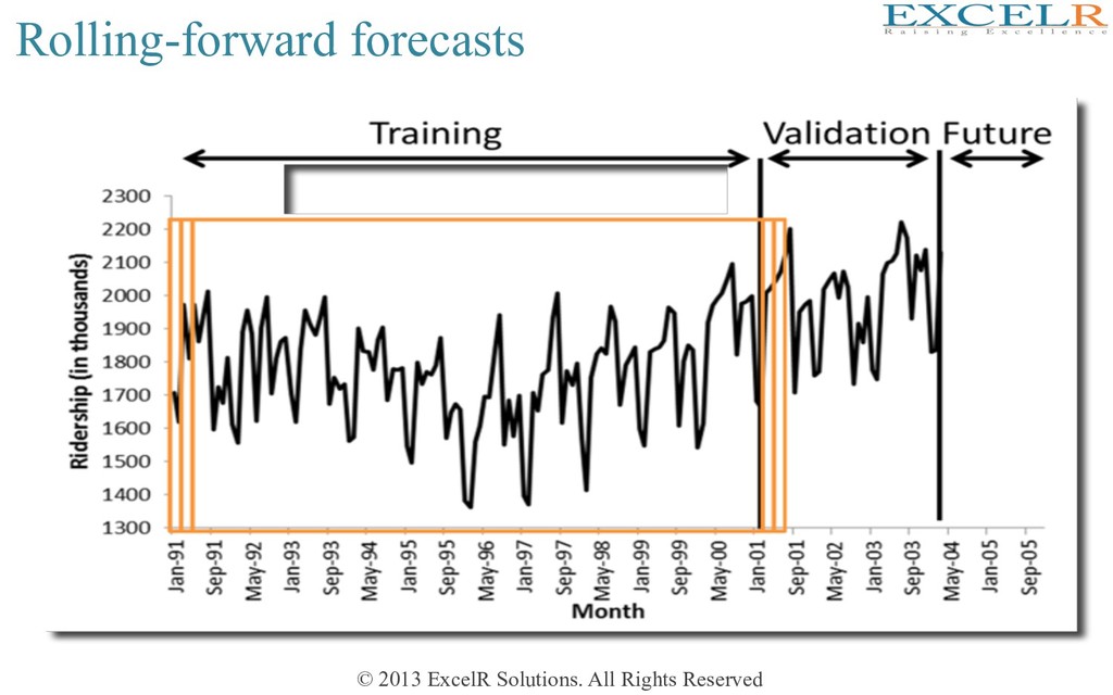
all historical data for forecas4ng ? Preliminaries for Step 3 of 8-Step forecasting strategy Training Data Valida4on Data Fit the model only to TRAINING period Assess performance on VALIDATION period Solu4on = DATA PARTIONING
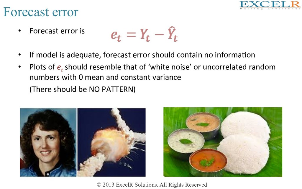
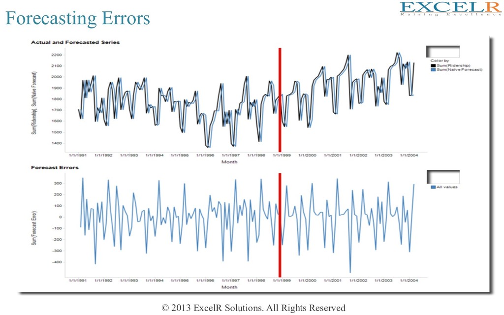
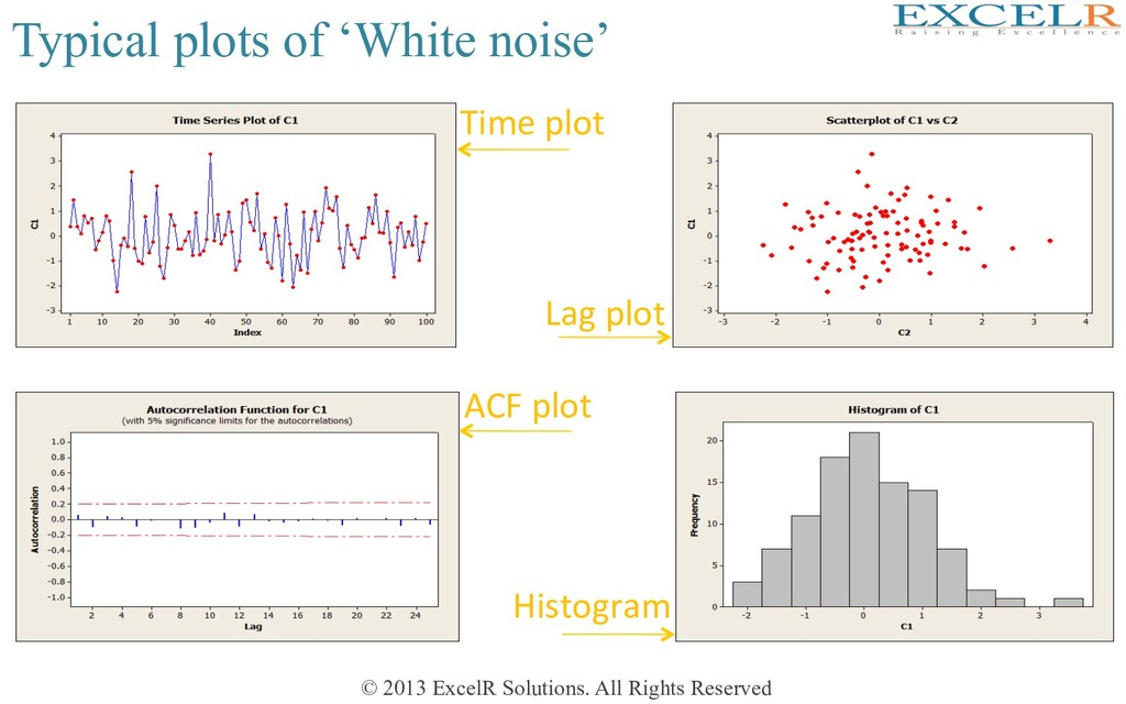
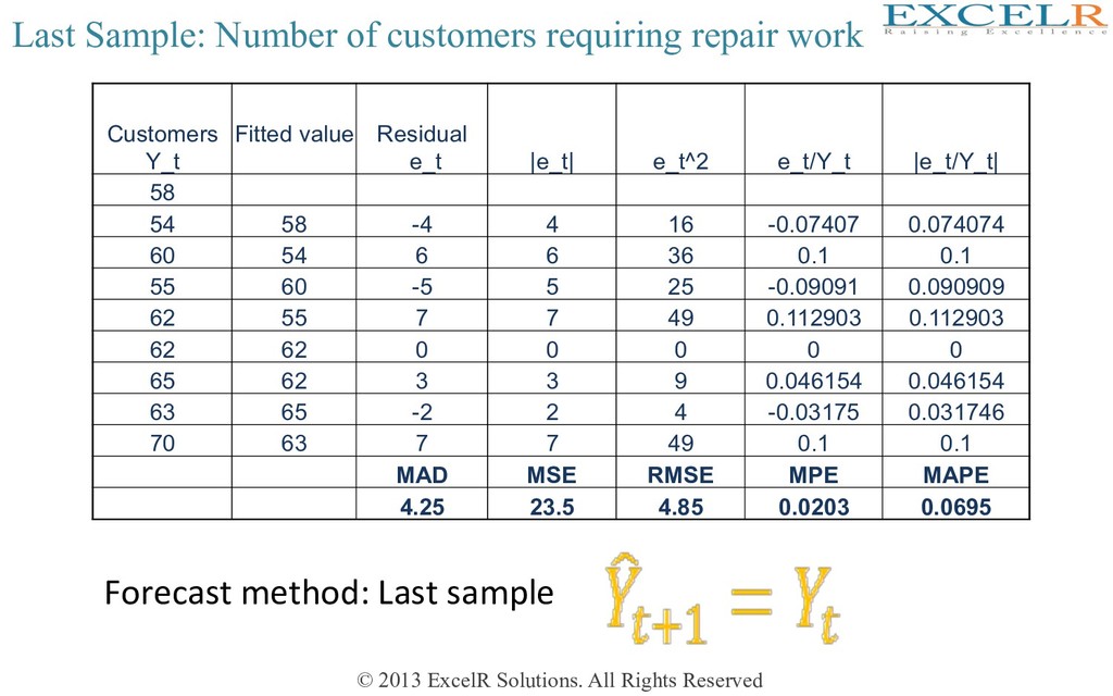
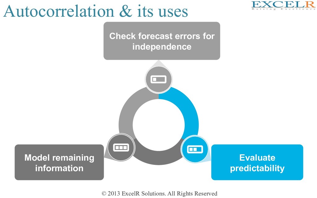
Forecast error is • If model is adequate, forecast error should contain no informaHon • Plots of et should resemble that of ‘white noise’ or uncorrelated random numbers with 0 mean and constant variance (There should be NO PATTERN)
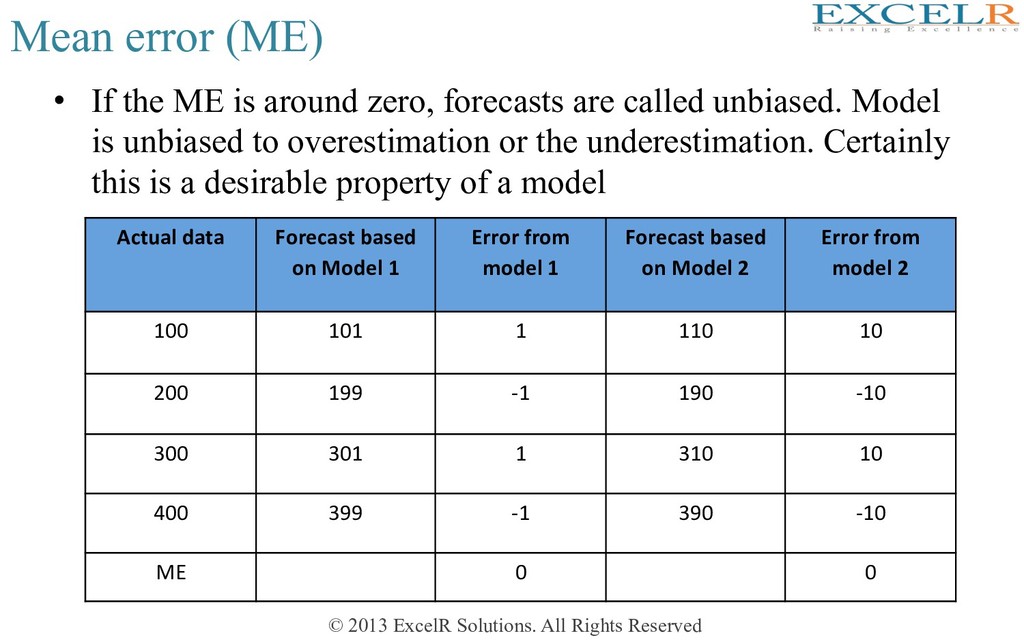
• If the ME is around zero, forecasts are called unbiased. Model is unbiased to overestimation or the underestimation. Certainly this is a desirable property of a model Actual data Forecast based on Model 1 Error from model 1 Forecast based on Model 2 Error from model 2 100 101 1 110 10 200 199 -1 190 -10 300 301 1 310 10 400 399 -1 390 -10 ME 0 0
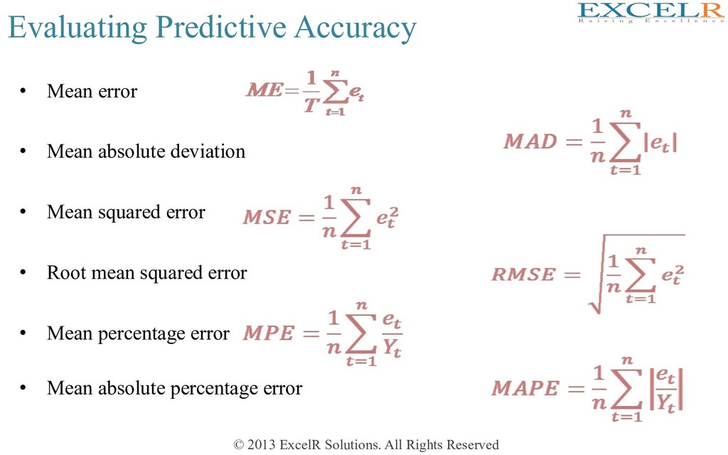
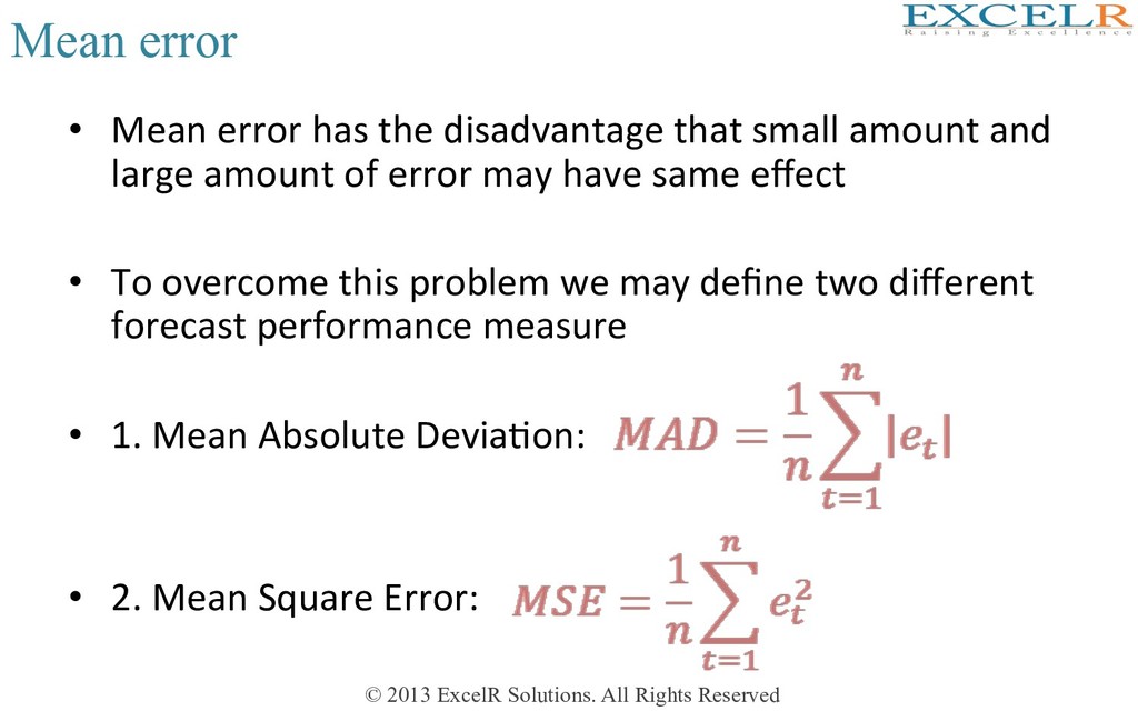
Mean error has the disadvantage that small amount and large amount of error may have same effect • To overcome this problem we may define two different forecast performance measure • 1. Mean Absolute DeviaHon: • 2. Mean Square Error:
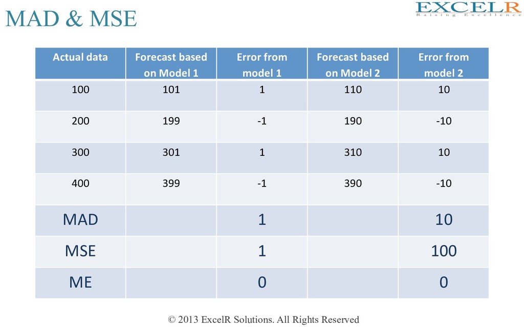
Actual data Forecast based on Model 1 Error from model 1 Forecast based on Model 2 Error from model 2 100 101 1 110 10 200 199 -1 190 -10 300 301 1 310 10 400 399 -1 390 -10 MAD 1 10 MSE 1 100 ME 0 0
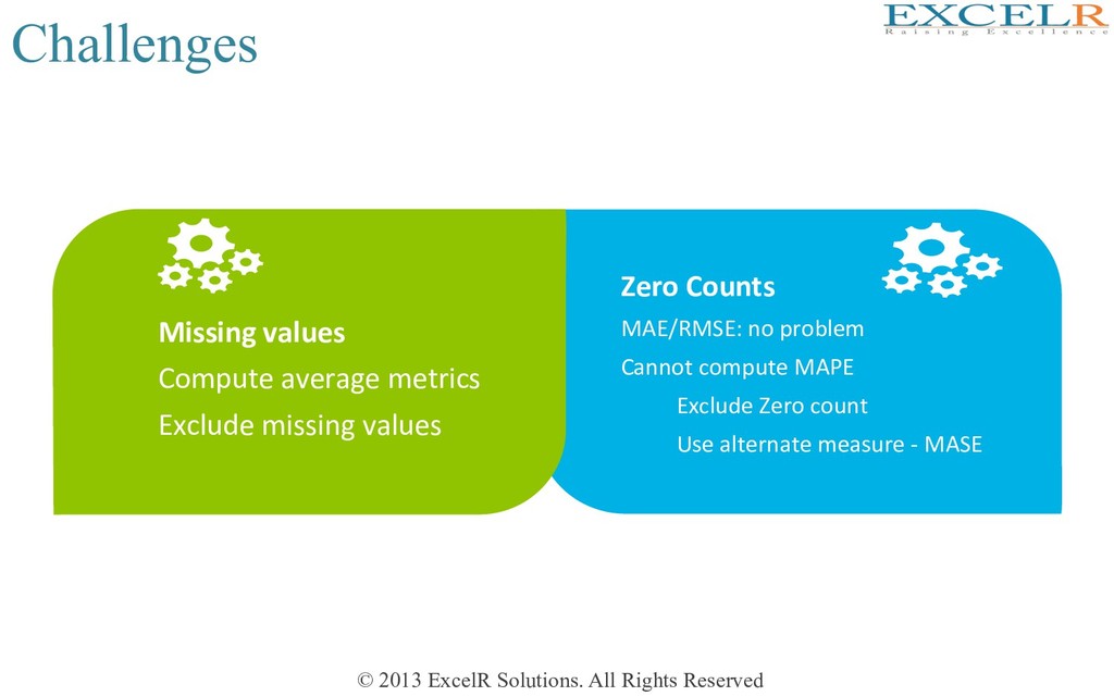
MAD, MSE • All these three measures are not unit free and also not scale free • Just think of a case that one is forecasHng sales figures. Someone in India using rupee figure, and somebody else in USA is expressing the same sales figure in dollar. Both are using the same model. However forecast measure will differ. This is a very awkward situaHon • MSE has the added disadvantage that its unit is in square. RMSE does not have this added disadvantage • So we need unit free measure
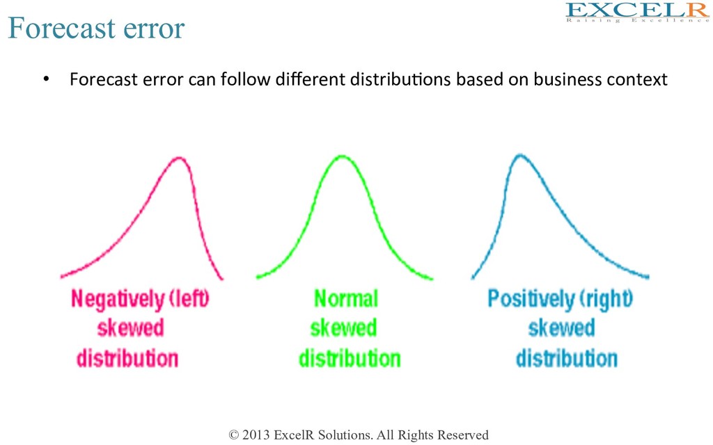
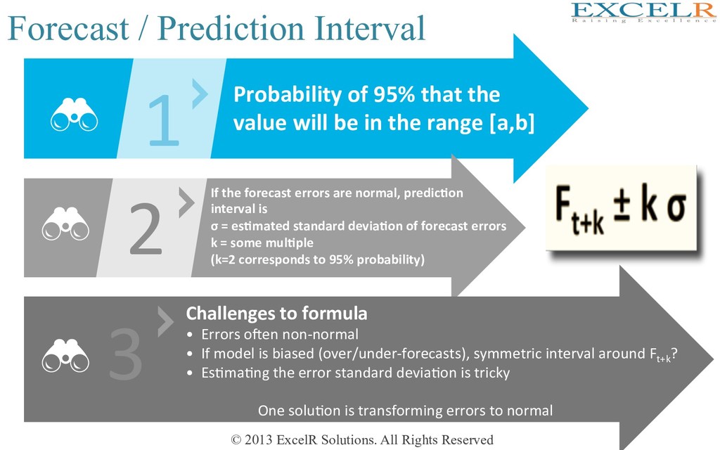
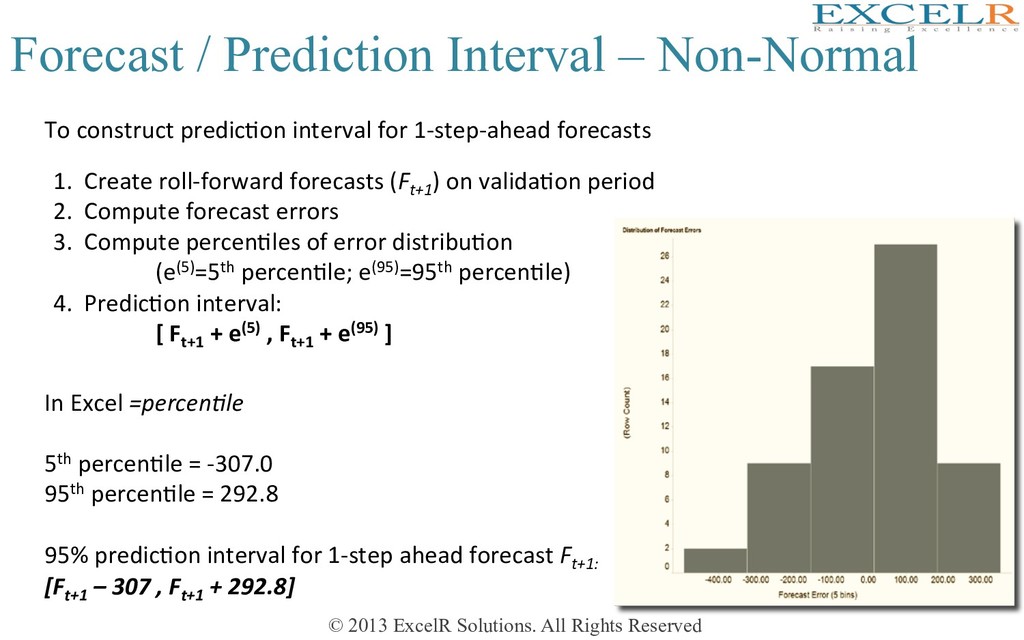
Interval 1 2 Probability of 95% that the value will be in the range [a,b] If the forecast errors are normal, predic4on interval is σ = es4mated standard devia4on of forecast errors k = some mul4ple (k=2 corresponds to 95% probability) 3 Challenges to formula • Errors ofen non-normal • If model is biased (over/under-forecasts), symmetric interval around Ft+k ? • EsHmaHng the error standard deviaHon is tricky One soluHon is transforming errors to normal
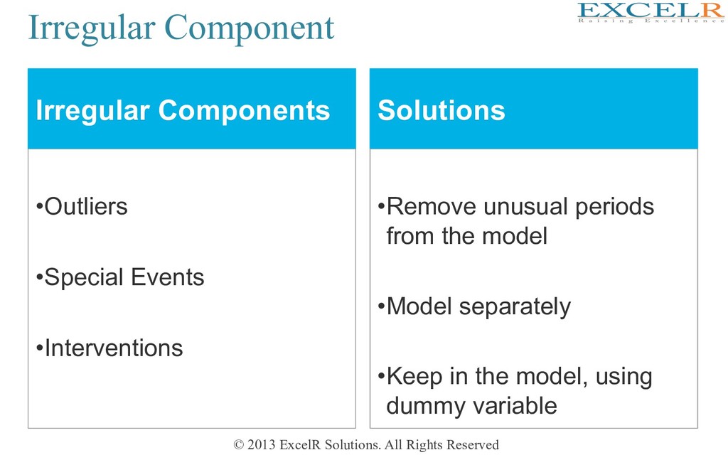
• Special Events • Interventions • Remove unusual periods from the model • Model separately • Keep in the model, using dummy variable Irregular Components Solutions
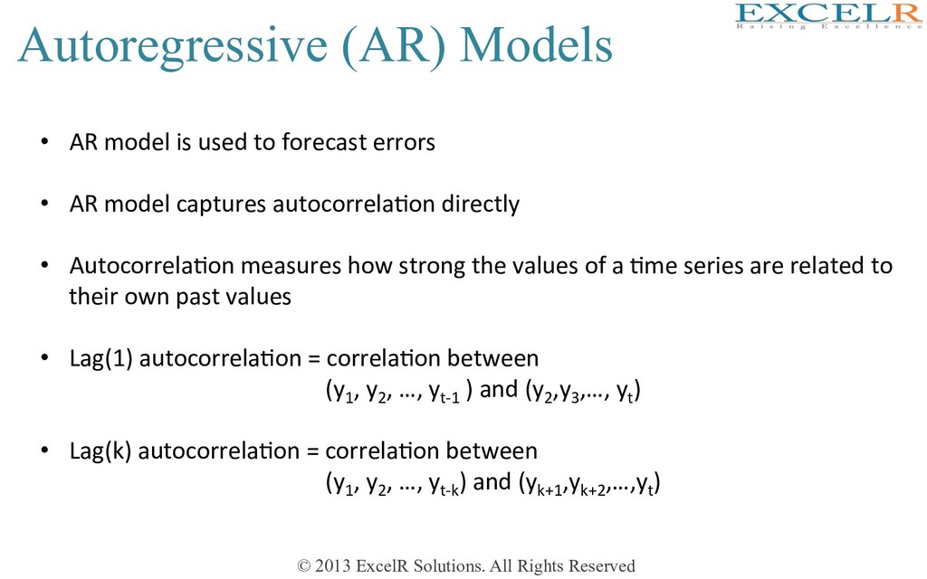
• AR model is used to forecast errors • AR model captures autocorrelaHon directly • AutocorrelaHon measures how strong the values of a Hme series are related to their own past values • Lag(1) autocorrelaHon = correlaHon between (y1 , y2 , …, yt-1 ) and (y2 ,y3 ,…, yt ) • Lag(k) autocorrelaHon = correlaHon between (y1 , y2 , …, yt-k ) and (yk+1 ,yk+2 ,…,yt )
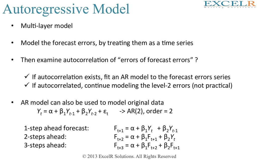
MulH-layer model • Model the forecast errors, by treaHng them as a Hme series • Then examine autocorrelaHon of “errors of forecast errors” ? ü If autocorrelaHon exists, fit an AR model to the forecast errors series ü If autocorrelated, conHnue modeling the level-2 errors (not pracHcal) • AR model can also be used to model original data Yt = α + β1 Yt-1 + β2 Yt-2 + εt -> AR(2), order = 2 1-step ahead forecast: Ft+1 = α + β1 Yt + β2 Yt-1 2-steps ahead: Ft+2 = α + β1 Ft+1 + β2 Yt 3-steps ahead: Ft+3 = α + β1 Ft+2 + β2 Ft+1
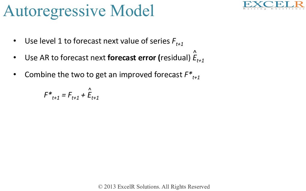
Use level 1 to forecast next value of series Ft+1 • Use AR to forecast next forecast error (residual) Et+1 • Combine the two to get an improved forecast F*t+1 F*t+1 = Ft+1 + Et+1 ^ ^
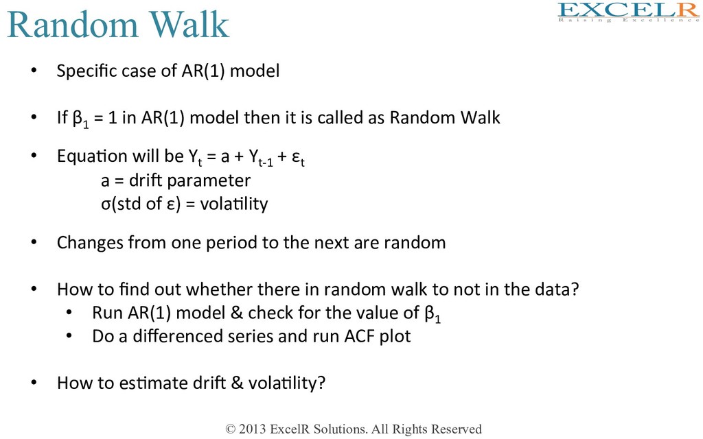
Specific case of AR(1) model • If β1 = 1 in AR(1) model then it is called as Random Walk • EquaHon will be Yt = a + Yt-1 + εt a = drif parameter σ(std of ε) = volaHlity • Changes from one period to the next are random • How to find out whether there in random walk to not in the data? • Run AR(1) model & check for the value of β1 • Do a differenced series and run ACF plot • How to esHmate drif & volaHlity?
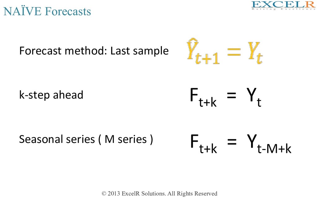
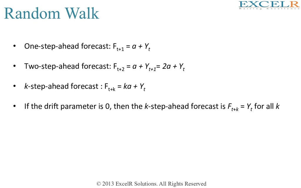
One-step-ahead forecast: Ft+1 = a + Yt • Two-step-ahead forecast: Ft+2 = a + Yt+1 = 2a + Yt • k-step-ahead forecast : Ft+k = ka + Yt • If the drif parameter is 0, then the k-step-ahead forecast is Ft+k = Yt for all k
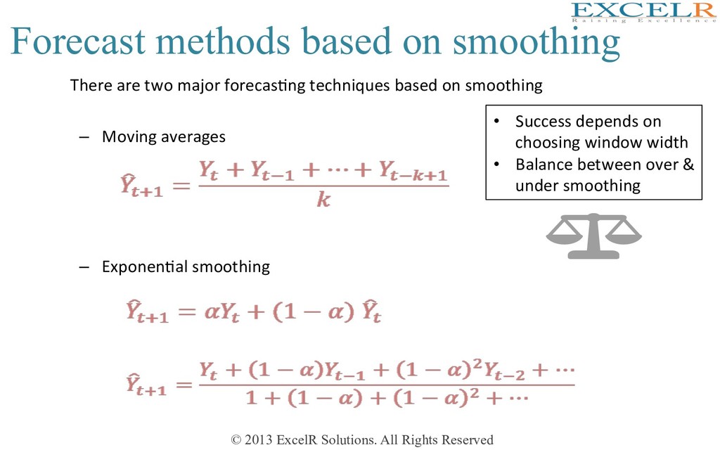
on smoothing There are two major forecasHng techniques based on smoothing – Moving averages – ExponenHal smoothing • Success depends on choosing window width • Balance between over & under smoothing
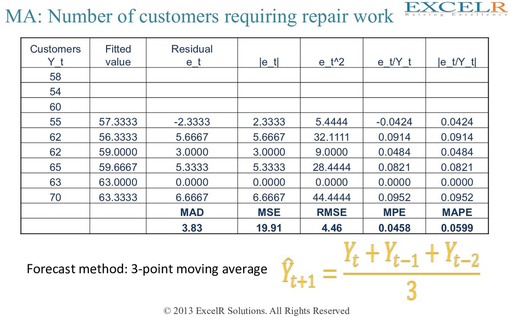
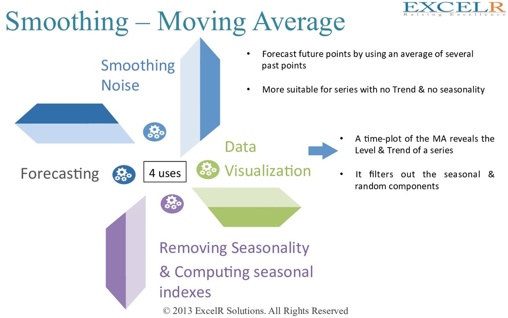
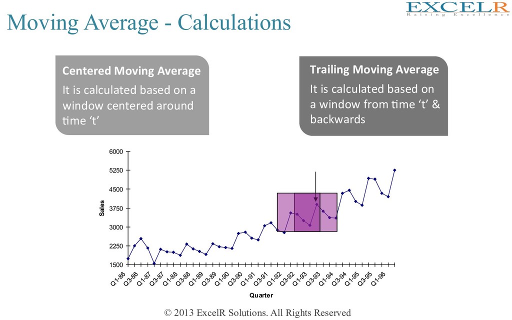
Average Smoothing Noise Data VisualizaHon Removing Seasonality & CompuHng seasonal indexes ForecasHng • Forecast future points by using an average of several past points • More suitable for series with no Trend & no seasonality 4 uses • A Hme-plot of the MA reveals the Level & Trend of a series • It filters out the seasonal & random components
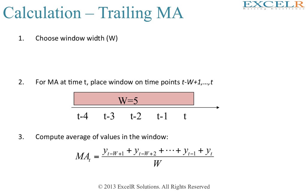
MA 1. Choose window width (W) 2. For MA at Hme t, place window on Hme points t-W+1,…,t 3. Compute average of values in the window: W y y y y MA t t W t W t t + + + + = − + − + − 1 2 1 ! t-4 t-3 t-2 t-1 t W=5
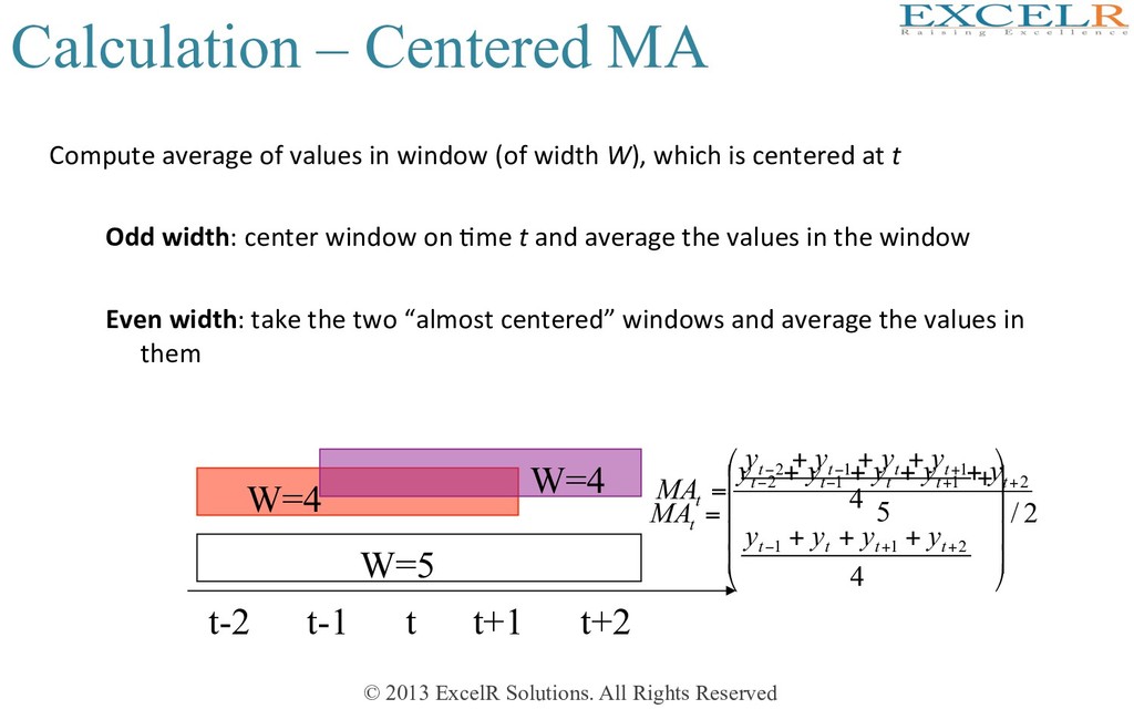
MA 5 2 1 1 2 + + − − + + + + = t t t t t t y y y y y MA 2 / 4 4 2 1 1 1 1 2 ⎟ ⎟ ⎟ ⎟ ⎠ ⎞ ⎜ ⎜ ⎜ ⎜ ⎝ ⎛ + + + + + + + = + + − + − − t t t t t t t t t y y y y y y y y MA Compute average of values in window (of width W), which is centered at t Odd width: center window on Hme t and average the values in the window Even width: take the two “almost centered” windows and average the values in them t-2 t-1 t t+1 t+2 W=5 W=4 W=4
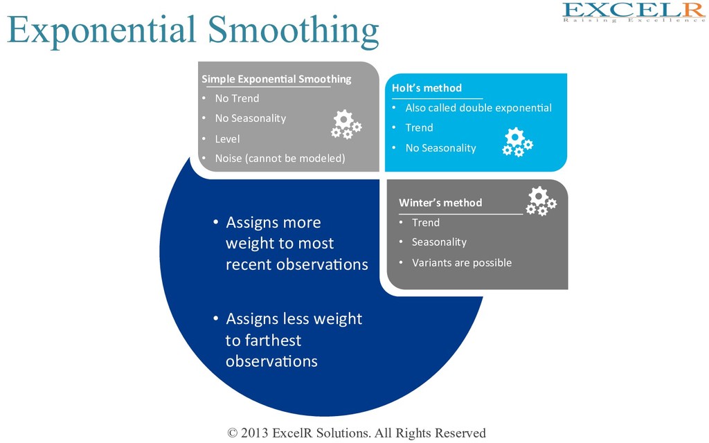
Assigns more weight to most recent observaHons • Assigns less weight to farthest observaHons Simple Exponen4al Smoothing • No Trend • No Seasonality • Level • Noise (cannot be modeled) Holt’s method • Also called double exponenHal • Trend • No Seasonality Winter’s method • Trend • Seasonality • Variants are possible
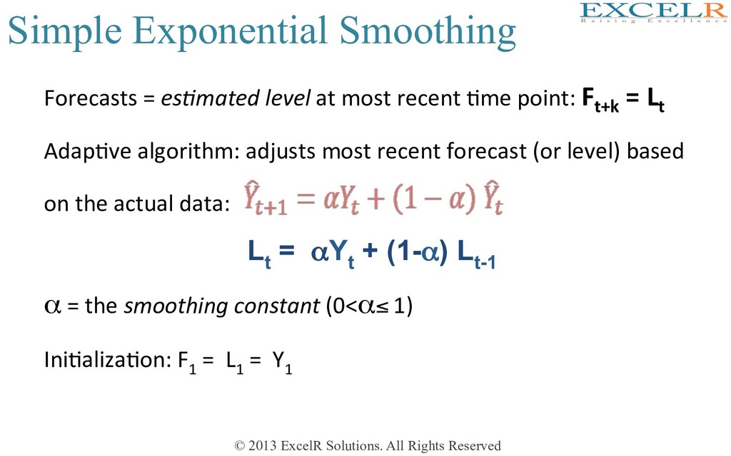
Forecasts = es+mated level at most recent Hme point: Ft+k = Lt AdapHve algorithm: adjusts most recent forecast (or level) based on the actual data: α = the smoothing constant (0<α≤ 1) IniHalizaHon: F 1 = L 1 = Y 1 L t = αY t + (1-α) L t-1
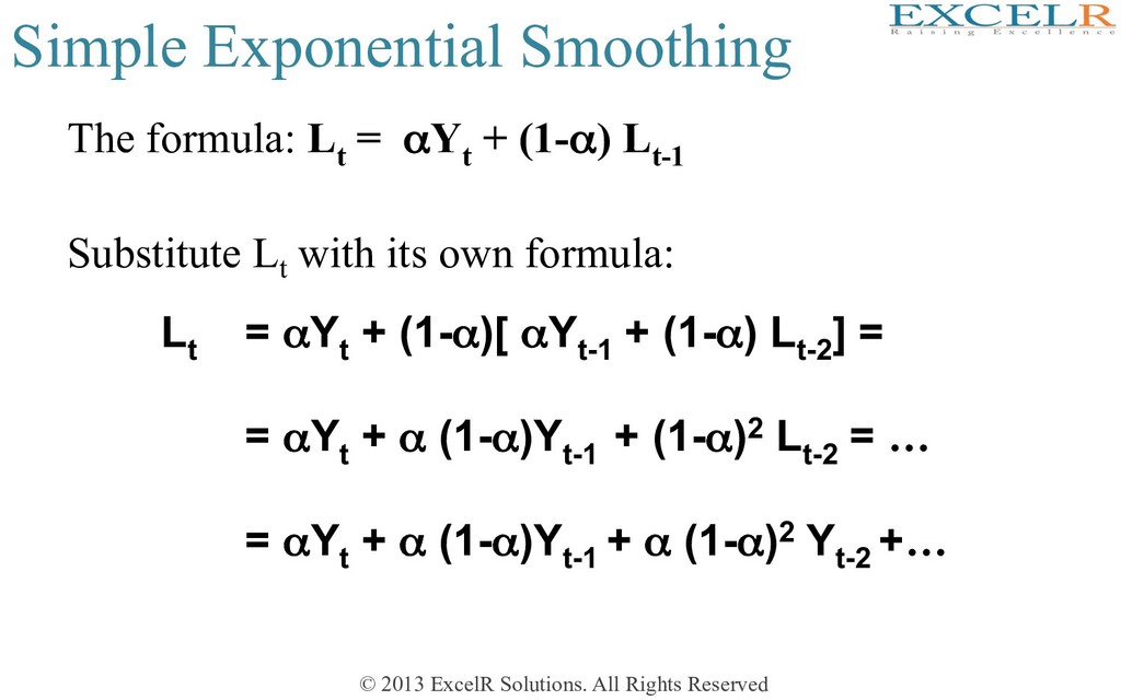
The formula: L t = αY t + (1-α) L t-1 Substitute Lt with its own formula: L t = αY t + (1-α)[ αY t-1 + (1-α) L t-2 ] = = αY t + α (1-α)Y t-1 + (1-α)2 L t-2 = … = αY t + α (1-α)Y t-1 + α (1-α)2 Y t-2 +…
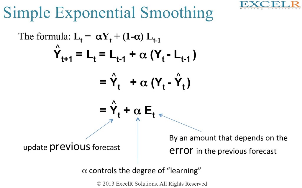
The formula: L t = αY t + (1-α) L t-1 Y t+1 = L t = L t-1 + α (Y t - L t-1 ) = Y t + α (Y t - Y t ) = Y t + α E t update previous forecast By an amount that depends on the error in the previous forecast α controls the degree of “learning” ^ ^ ^ ^
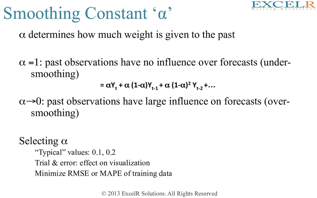
α determines how much weight is given to the past α =1: past observations have no influence over forecasts (under- smoothing) α→0: past observations have large influence on forecasts (over- smoothing) Selecting α “Typical” values: 0.1, 0.2 Trial & error: effect on visualization Minimize RMSE or MAPE of training data = αY t + α (1-α)Y t-1 + α (1-α)2 Y t-2 +…
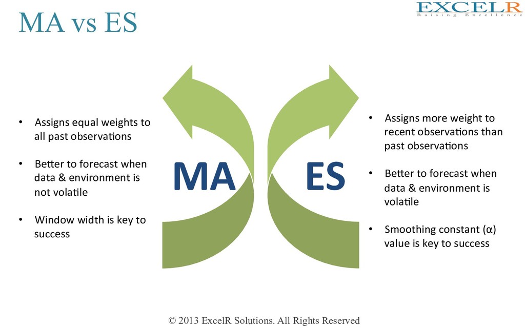
MA ES • Assigns equal weights to all past observaHons • BeKer to forecast when data & environment is not volaHle • Window width is key to success • Assigns more weight to recent observaHons than past observaHons • BeKer to forecast when data & environment is volaHle • Smoothing constant (α) value is key to success
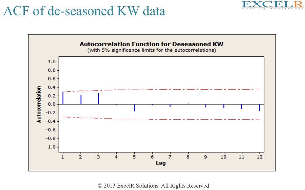
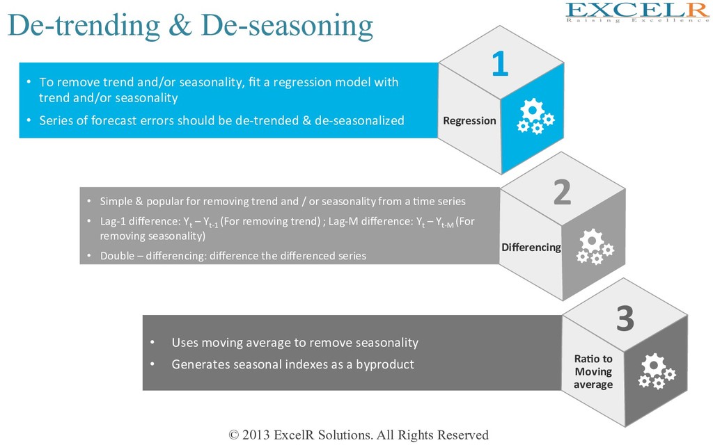
• Simple & popular for removing trend and / or seasonality from a Hme series • Lag-1 difference: Yt – Yt-1 (For removing trend) ; Lag-M difference: Yt – Yt-M (For removing seasonality) • Double – differencing: difference the differenced series • Uses moving average to remove seasonality • Generates seasonal indexes as a byproduct • To remove trend and/or seasonality, fit a regression model with trend and/or seasonality • Series of forecast errors should be de-trended & de-seasonalized 1 Regression Ra4o to Moving average 3 2 Differencing
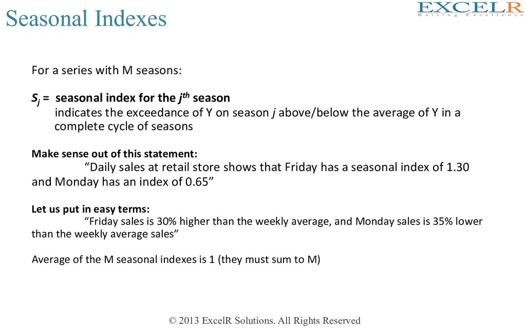
a series with M seasons: Sj = seasonal index for the jth season indicates the exceedance of Y on season j above/below the average of Y in a complete cycle of seasons Make sense out of this statement: “Daily sales at retail store shows that Friday has a seasonal index of 1.30 and Monday has an index of 0.65” Let us put in easy terms: “Friday sales is 30% higher than the weekly average, and Monday sales is 35% lower than the weekly average sales” Average of the M seasonal indexes is 1 (they must sum to M)
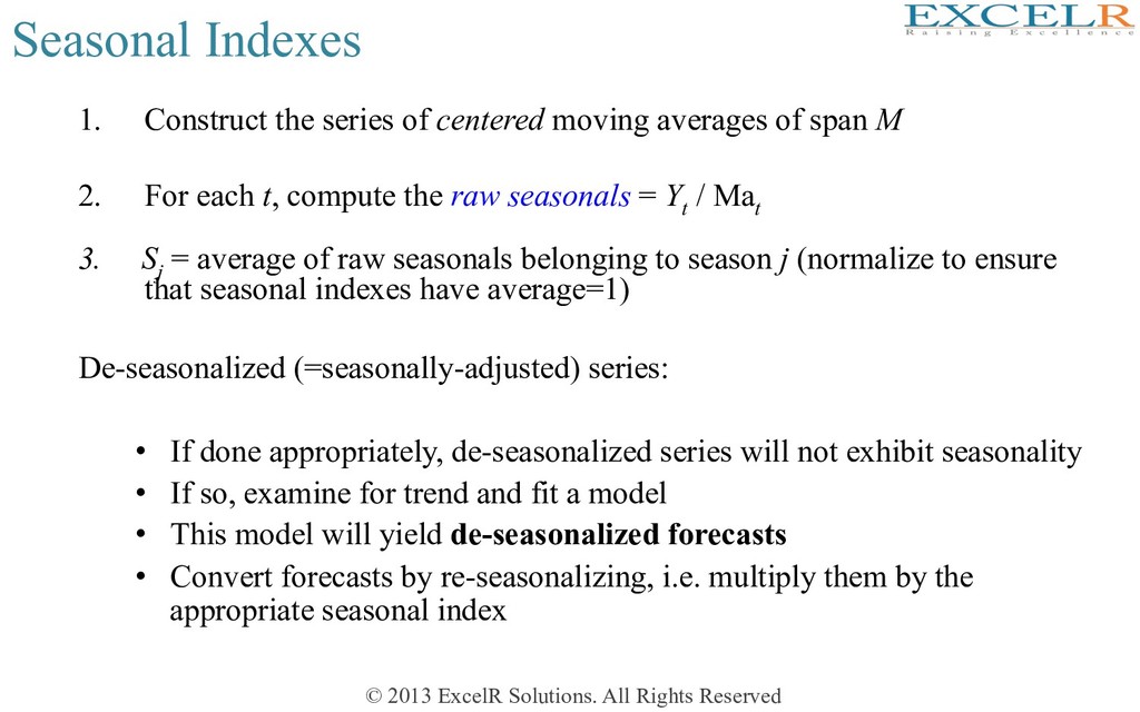
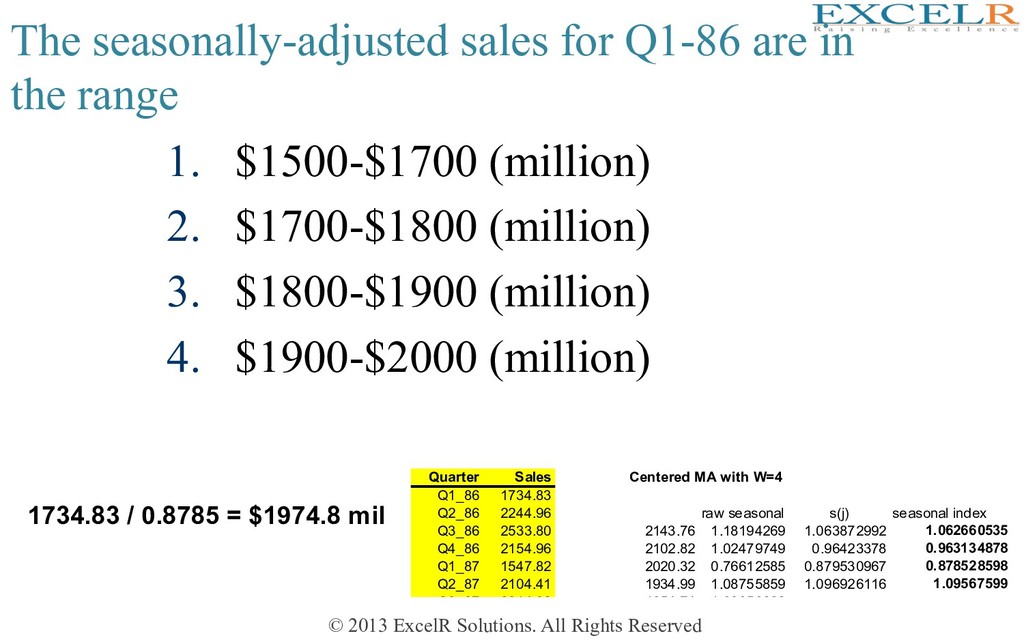
Construct the series of centered moving averages of span M 2. For each t, compute the raw seasonals = Y t / Ma t 3. S j = average of raw seasonals belonging to season j (normalize to ensure that seasonal indexes have average=1) De-seasonalized (=seasonally-adjusted) series: • If done appropriately, de-seasonalized series will not exhibit seasonality • If so, examine for trend and fit a model • This model will yield de-seasonalized forecasts • Convert forecasts by re-seasonalizing, i.e. multiply them by the appropriate seasonal index
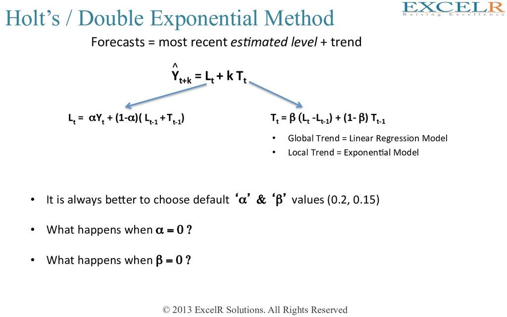
Exponential Method Forecasts = most recent es+mated level + trend Yt+k = Lt + k Tt ^ L t = αY t + (1-α)( L t-1 + T t-1 ) Tt = β (Lt -Lt-1 ) + (1- β) Tt-1 • Global Trend = Linear Regression Model • Local Trend = ExponenHal Model • It is always beKer to choose default ‘α’ & ‘β’ values (0.2, 0.15) • What happens when α = 0 ? • What happens when β = 0 ?
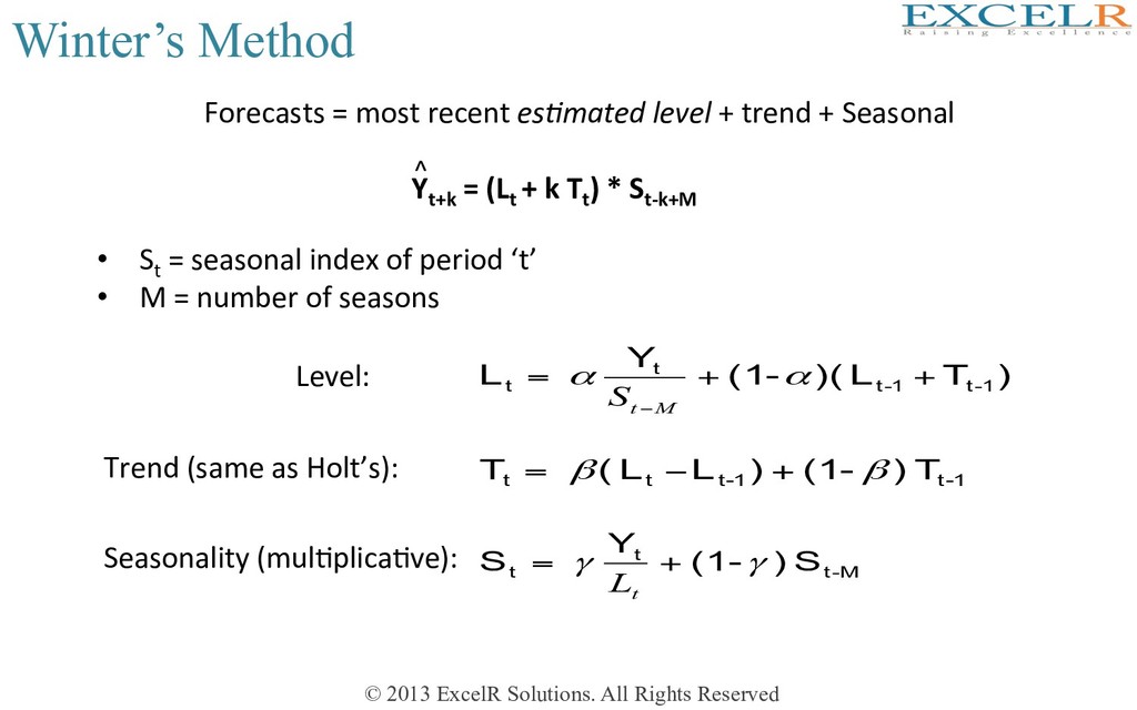
= most recent es+mated level + trend + Seasonal Yt+k = (Lt + k Tt ) * St-k+M ^ • St = seasonal index of period ‘t’ • M = number of seasons Level: Trend (same as Holt’s): Seasonality (mulHplicaHve): ) T L )( (1- Y L 1 - t 1 - t t t + + = − α α M t S 1 - t 1 - t t t T ) (1- ) L L ( T β β + − = -M t t t S ) (1- Y S γ γ + = t L
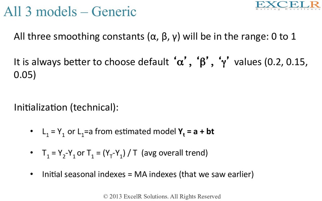
– Generic IniHalizaHon (technical): • L 1 = Y 1 or L 1 =a from esHmated model Yt = a + bt • T 1 = Y 2 -Y 1 or T 1 = (Y T -Y 1 ) / T (avg overall trend) • IniHal seasonal indexes = MA indexes (that we saw earlier) All three smoothing constants (α, β, γ) will be in the range: 0 to 1 It is always beKer to choose default ‘α’, ‘β’, ‘γ’ values (0.2, 0.15, 0.05)
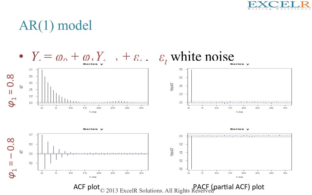
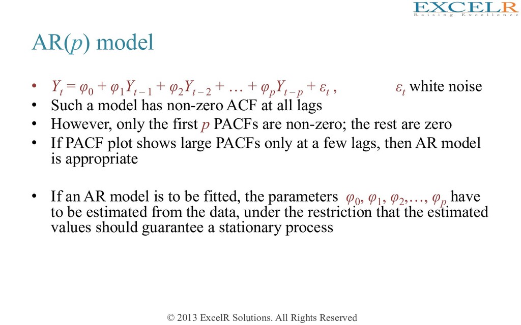
Yt = φ0 + φ1 Yt – 1 + φ2 Yt – 2 + … + φp Yt – p + εt , εt white noise • Such a model has non-zero ACF at all lags • However, only the first p PACFs are non-zero; the rest are zero • If PACF plot shows large PACFs only at a few lags, then AR model is appropriate • If an AR model is to be fitted, the parameters φ0 , φ1 , φ2 ,…, φp have to be estimated from the data, under the restriction that the estimated values should guarantee a stationary process
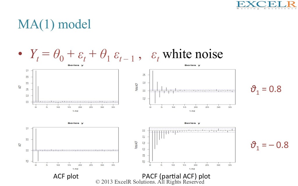
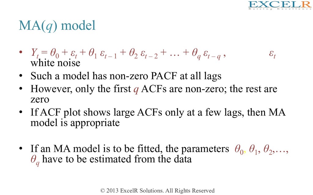
Yt = θ0 + εt + θ1 εt – 1 + θ2 εt – 2 + … + θq εt – q , εt white noise • Such a model has non-zero PACF at all lags • However, only the first q ACFs are non-zero; the rest are zero • If ACF plot shows large ACFs only at a few lags, then MA model is appropriate • If an MA model is to be fitted, the parameters θ0 , θ1 , θ2 ,…, θq have to be estimated from the data
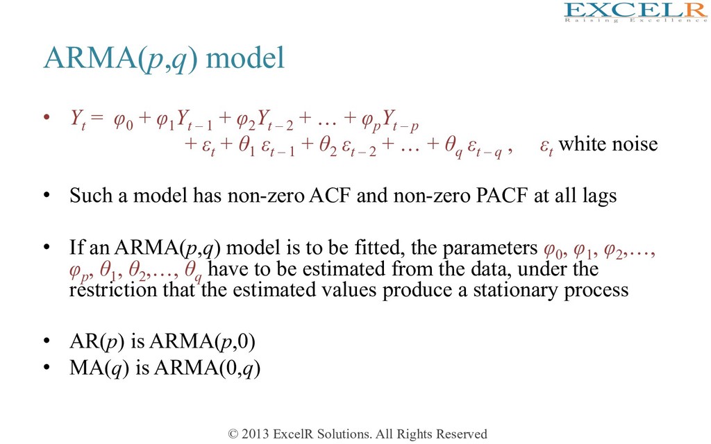
Yt = φ0 + φ1 Yt – 1 + φ2 Yt – 2 + … + φp Yt – p + εt + θ1 εt – 1 + θ2 εt – 2 + … + θq εt – q , εt white noise • Such a model has non-zero ACF and non-zero PACF at all lags • If an ARMA(p,q) model is to be fitted, the parameters φ0 , φ1 , φ2 ,…, φp , θ1 , θ2 ,…, θq have to be estimated from the data, under the restriction that the estimated values produce a stationary process • AR(p) is ARMA(p,0) • MA(q) is ARMA(0,q)
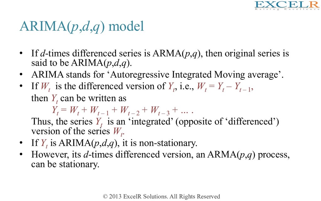
If d-times differenced series is ARMA(p,q), then original series is said to be ARIMA(p,d,q). • ARIMA stands for ‘Autoregressive Integrated Moving average’. • If Wt is the differenced version of Yt , i.e., Wt = Yt – Yt – 1 , then Yt can be written as Yt = Wt + Wt – 1 + Wt – 2 + Wt – 3 + … . Thus, the series Yt is an ‘integrated’ (opposite of ‘differenced’) version of the series Wt . • If Yt is ARIMA(p,d,q), it is non-stationary. • However, its d-times differenced version, an ARMA(p,q) process, can be stationary.
• Model identification – If the time plot ‘looks’ non-stationary, difference it until the plot looks stationary – Look at ACF and PACF plots for possible clue on model order (p, q) – When in doubt (regarding choice of p and q), use the principle of parsimony: A simple model is better than a complex model • Estimate model parameters • Check residuals for health of model • Iterate if necessary • Forecast using the fitted model