data_science_course_singapore.pdf

Transcript

1. Forecasting Time Series
2. © 2013 ExcelR Solutions. All Rights Reserved My Introduction PMP PMI-ACP PMI-RMP CSM LSSGB Project Management Professional Agile Cer4fied Prac44oner Risk Management Professional Cer4fied Scrum Master Lean Six Sigma Green Belt LSSBB SSMBB ITIL Lean Six Sigma Black Belt Six Sigma Master Black Belt Informa4on Technology Infrastructure Library Agile PM Dynamic System Development Methodology Atern Name: Bharani Kumar Educa+on: IIT Hyderabad Indian School of Business Professional cer+fica+ons:
3. © 2013 ExcelR Solutions. All Rights Reserved My Introduction HSBC Driven using UK policies ITC Infotech Driven using Indian policies SME Infosys Driven using Indian policies under Large enterprises DeloiHe Driven using US policies 1 2 3 4 RESEARCH in ANALYTICS, DEEP LEARNING & IOT DATA SCIENTIST
4. Why Forecas4ng Learn about the various examples of forecasHng Forecas4ng Strategy Learn about decomposing, forecasHng & combining EDA & Graphical Representa4on Learn about exploratory data analysis, scaKer plot, Hme plot, lag plot, ACF plot Forecas4ng components Learn about Level, Trend, Seasonal, Cyclical, Random components Forecas4ng Models & Errors Learn about various forecasHng models to be discussed & the various error measures AGENDA Why Forecas4ng? Forecas4ng Strategy EDA & Graphical Representa4on Forecas4ng Decomposi4on components AGENDA
5. © 2013 ExcelR Solutions. All Rights Reserved Why Forecasting •  Why forecast, when you would know the outcome eventually? •  Early knowledge is the key, even if that knowledge is imperfect –  For seQng producHon schedules, one needs to forecast sales –  For staffing of call centers, a company needs to forecast the demand for service –  For dealing with epidemic emergencies, naHons should forecast the various flu
6. © 2013 ExcelR Solutions. All Rights Reserved Types of forecast Micro Scale or Macro Scale Qualita4ve or Quan4ta4ve Short Term or Long Term Data or Judgment Forecas4ng Classifica4on Point Forecast Density Forecast Interval Forecast
7. © 2013 ExcelR Solutions. All Rights Reserved Who generates Forecast?
8. © 2013 ExcelR Solutions. All Rights Reserved Who generates Forecast?
9. © 2013 ExcelR Solutions. All Rights Reserved Time series vs Cross-sectional data 01 Cross-sec4onal Data 02 Time Series Data
10. © 2013 ExcelR Solutions. All Rights Reserved Dataset for further discussion Monthly FooWalls of customers from Jan 1991 to March 2004 t = 1, 2, 3,…....= Hme period index Yt = value of the series at Hme period t Yt+k = forecast for Hme period t+k, given data unHl Hme t et = forecast error for period t Month Footfall in thousands Jan-91 1709 Feb-91 1621 Mar-91 1973 Apr-91 1812 May-91 1975 Jun-91 1862 Jul-91 1940 Aug-91 2013 Sep-91 1596 Oct-91 1725 Nov-91 1676 Dec-91 1814 Jan-92 1615 Feb-92 1557 Mar-92 1891 Apr-92 1956 May-92 1885 Jun-92 1623
11. © 2013 ExcelR Solutions. All Rights Reserved Forecasting Strategy 01 02 03 04 05 Define Goal Data Collec4on Explore & Visualize Series Pre-Process Data Par44on Series 06 07 08 Apply Forecas4ng Method(s) Evaluate & Compare Performance Implement Forecasts / System
12. © 2013 ExcelR Solutions. All Rights Reserved Forecasting Strategy – Step 1 • DescripHve = Time Series Analysis • PredicHve = Time Series ForecasHng • How far into the future? k in Yt+k • Rolling forward or at single Hme point? #1 Is the goal descriptive or predictive? #2 What is the forecast horizon? • Who are the stakeholders? • Numerical or event forecast? • Cost of over-predicHon & under-predicHon • In-house forecasHng or consultants? • How many series? How ofen? • Data & sofware availability #3 How will the forecast be used? #4 Forecasting expertise & automation Define Goal
13. © 2013 ExcelR Solutions. All Rights Reserved Forecasting Strategy – Step 2 • Typically small sample, so need good quality • Data same as series to be forecasted • Should we use real-Hme Hcket collecHon data? • Balance between signal & noise • AggregaHon / DisaggregaHon #1 Data Quality #2 Temporal Frequency • Coverage of the data – Geographical, populaHon, Hme,… • Should be aligned with goal • Necessary informaHon source • Affects modeling process from start to end • Level of communicaHon/ coordinaHon between forecasters & domain experts #3 Series Granularity? #4. Domain exper4se Data Collec-on
14. © 2013 ExcelR Solutions. All Rights Reserved Forecasting Strategy Step3 (Explore Series) Seasonal PaHerns SYSTEMATIC PART Level Trend Season al PaHern s NON-SYSTEMATIC PART Noise Addi4ve: Yt = Level + Trend + Seasonality + Noise Mul4plica4ve: Yt = Level x Trend x Seasonality x Noise
15. © 2013 ExcelR Solutions. All Rights Reserved Trend Component •  Persistent, overall upward or downward paKern •  Due to populaHon, technology etc. •  Overall Upward or Downward Movement •  Several years duraHon Mo., Qtr., Yr. Response
16. © 2013 ExcelR Solutions. All Rights Reserved Seasonal Component •  Regular paKern of up & down fluctuaHons •  Due to weather, customs etc. •  Occurs within one year •  Example: Passenger traffic during 24 hours Mo., Qtr. Response Summer
17. © 2013 ExcelR Solutions. All Rights Reserved Irregular/Random/Noise Component •  ErraHc, unsystemaHc, ‘residual’ fluctuaHons •  Due to random variaHon or unforeseen events –  Union strike –  War •  Short duraHon & nonrepeaHng
18. © 2013 ExcelR Solutions. All Rights Reserved Time Series Components
19. © 2013 ExcelR Solutions. All Rights Reserved Time Plot •  Plots a variable against Hme index •  Appropriate for visualizing serially collected data (Hme series) •  Brings out many useful aspects of the structure of the data •  Example: Electrical usage for Washington Water Power (Quarterly data from 1980 to 1991)
20. © 2013 ExcelR Solutions. All Rights Reserved Time plot 400 500 600 700 800 900 1000 1100 1980 1982 1984 1986 1988 1990 Power usage (KilowaHs) Year Electrical power usage for Washington Water Power: 1980-1991
21. © 2013 ExcelR Solutions. All Rights Reserved Observations •  There is a cyclic trend •  Maximum demand in first quarter; minimum in third quarter •  There may also be a slowly increasing trend (to be examined) •  Any reasonable forecast should have cyclic fluctuaHons •  Trend (if any) need to be uHlized for forecasHng •  Forecast would not be exact – there would be some error
22. © 2013 ExcelR Solutions. All Rights Reserved Time plot
23. © 2013 ExcelR Solutions. All Rights Reserved Quarterly Sales of Ice-cream
24. © 2013 ExcelR Solutions. All Rights Reserved Scatter Diagram •  Plots one variable against another •  One of the simplest tools for visualizaHon Cost Age 859 8 682 5 471 3 708 9 1094 11 224 2 320 1 651 8 1049 12 ž  Example: Maintenance cost and Age for nine buses (Spokane Transit) ž  This is an example of cross-secHonal data (observaHons collected in a single point of Hme)
25. © 2013 ExcelR Solutions. All Rights Reserved Scatter Plot 0 200 400 600 800 1000 1200 0 2 4 6 8 10 12 14 Yearly cost of maintenance (US $) Age of bus
26. © 2013 ExcelR Solutions. All Rights Reserved Observations •  Older buses have higher cost of maintenance •  There is some variaHon (case to case) •  The rise in cost is about $ 80 per year of age •  It may be possible to use ‘age’ to forecast maintenance cost •  Forecast would not be a ‘certain’ predicHon – there would be some error
27. © 2013 ExcelR Solutions. All Rights Reserved Lag plot •  Plots a variable against its own lagged sample •  Brings out possible associaHon between successive samples •  Example: Monthly sale of VCRs by a music store in a year = Number of VCRs sold in Hme period t = Number of VCRs sold in Hme period t – k
28. © 2013 ExcelR Solutions. All Rights Reserved Example of lagged variables Number of VCRs sold in a month Time Original Lagged one step Lagged two steps 1 123 2 130 123 3 125 130 123 4 138 125 130 5 145 138 125 6 142 145 138 7 141 142 145 8 146 141 142 9 147 146 141 10 157 147 146 11 150 157 147 12 160 150 157
29. © 2013 ExcelR Solutions. All Rights Reserved Lag plot (k = 1) 120 125 130 135 140 145 150 155 160 120 125 130 135 140 145 150 155 160 ScaHer plot of VCR sales with 1-step lagged VCR sales
30. © 2013 ExcelR Solutions. All Rights Reserved Observations •  There is a reasonable degree of associaHon between the original variable and the lagged one •  Value of lagged variable is known beforehand, so it is useful for predicHon •  AssociaHon between original and lagged variable may be quan+fied through a correlaHon
31. © 2013 ExcelR Solutions. All Rights Reserved Autocorrelation •  CorrelaHon between a variable and its lagged version (one Hme-step or more) = ObservaHon in Hme period t = ObservaHon in Hme period t – k = Mean of the values of the series = AutocorrelaHon coefficient for k-step lag
32. © 2013 ExcelR Solutions. All Rights Reserved Standard error of rk •  The standard error is •  Increases progressively with k, but eventually reaches a maximum value •  If the ‘true’ autocorrelaHon is 0, then the esHmate rk should be in the interval (– 2SE(rk ), 2SE(rk )) 95% of the Hme •  SomeHmes SE(rk ) is approximated by The standard error of the mean esHmates the variability between samples whereas the standard deviaHon measures the variability within a single sample.
33. © 2013 ExcelR Solutions. All Rights Reserved Correlogram or ACF plot •  Plots the ACF or AutocorrelaHon funcHon (rk ) against the lag (k) •  Plus-and-minus two-standard errors are displayed as limits to be exceeded for staHsHcal significance •  Reveals lagged variables that can be potenHally useful for forecasHng
34. © 2013 ExcelR Solutions. All Rights Reserved Correlogram for VCR data
35. © 2013 ExcelR Solutions. All Rights Reserved ACF plot for electricity usage data
36. © 2013 ExcelR Solutions. All Rights Reserved Observations •  Every alternate sample is large, many of them staHsHcally significant also •  ACFs at lags 4, 8, 12, etc are posiHve •  ACF at lags 2,6,10 etc are negaHve •  All these pick up the seasonal aspect of the data •  The data may be re-examined afer ‘removing’ seasonality
37. © 2013 ExcelR Solutions. All Rights Reserved ACF of de-seasoned KW data
38. © 2013 ExcelR Solutions. All Rights Reserved Observations •  De-seasoned series has small ACFs •  This part of the data has liKle forecasHng value
39. © 2013 ExcelR Solutions. All Rights Reserved Typical questions in exploratory analysis All the plots contain informaHon regarding these quesHons Is there a TREND? Is there a SEASONALITY? Are the data RANDOM?
40. © 2013 ExcelR Solutions. All Rights Reserved Time series plots
41. © 2013 ExcelR Solutions. All Rights Reserved Effect of omission of data on the Time series plot
42. © 2013 ExcelR Solutions. All Rights Reserved Effect of omission of data on the Time series plot
43. © 2013 ExcelR Solutions. All Rights Reserved Confusing kind of trend due to other type of scaling 0 20 40 60 80 y 0 5 10 15 20 t 0 20 40 60 80 y 0 1 2 3 Log t 2.5 3 3.5 4 4.5 Log y 0 5 10 15 20 t 2.5 3 3.5 4 4.5 Log y 0 1 2 3 Log t
44. © 2013 ExcelR Solutions. All Rights Reserved Few points on Plots Plot helps us to summarize & reveal paKerns in data Graphics help us to idenHfy anomalies in data Plot helps us to present a huge amount of data in small space & makes huge data set coherent To get all the advantages of plot, the “Aspect RaHo” of plot is very crucial The raHo of Height to Width of a plot is called the ASPECT RATIO
45. © 2013 ExcelR Solutions. All Rights Reserved Aspect Ratio •  Generally aspect raHo should be around 0.618 •  However, for long Hme series data aspect raHo should be around 0.25. To understand the impact of aspect raHo see the two plots in the next two slides
46. © 2013 ExcelR Solutions. All Rights Reserved Aspect ratio
47. © 2013 ExcelR Solutions. All Rights Reserved Aspect ratio
48. © 2013 ExcelR Solutions. All Rights Reserved Should we use all historical data for forecas4ng ? Preliminaries for Step 3 of 8-Step forecasting strategy Training Data Valida4on Data Fit the model only to TRAINING period Assess performance on VALIDATION period Solu4on = DATA PARTIONING
49. © 2013 ExcelR Solutions. All Rights Reserved Partitioning Deploy model by joining Training + ValidaHon to forecast the Future
50. © 2013 ExcelR Solutions. All Rights Reserved How to choose a Validation Period? Forecast Horizon Seasonality Length of series Underlying condi4ons affec4ng series Strategy to choose Valida4on Data Period
51. © 2013 ExcelR Solutions. All Rights Reserved Rolling-forward forecasts
52. © 2013 ExcelR Solutions. All Rights Reserved NAÏVE Forecasts Forecast method: Last sample k-step ahead Seasonal series ( M series ) Ft+k = Yt Ft+k = Yt-M+k
53. © 2013 ExcelR Solutions. All Rights Reserved Forecast error •  Forecast error is •  If model is adequate, forecast error should contain no informaHon •  Plots of et should resemble that of ‘white noise’ or uncorrelated random numbers with 0 mean and constant variance (There should be NO PATTERN)
54. © 2013 ExcelR Solutions. All Rights Reserved Forecast error •  Forecast error can follow different distribuHons based on business context
55. © 2013 ExcelR Solutions. All Rights Reserved Forecasting Errors
56. © 2013 ExcelR Solutions. All Rights Reserved Evaluating Predictive Accuracy •  Mean error •  Mean absolute deviation •  Mean squared error •  Root mean squared error •  Mean percentage error •  Mean absolute percentage error
57. © 2013 ExcelR Solutions. All Rights Reserved Typical plots of ‘White noise’ Time plot Lag plot ACF plot Histogram
58. © 2013 ExcelR Solutions. All Rights Reserved Mean error (ME) •  If the ME is around zero, forecasts are called unbiased. Model is unbiased to overestimation or the underestimation. Certainly this is a desirable property of a model Actual data Forecast based on Model 1 Error from model 1 Forecast based on Model 2 Error from model 2 100 101 1 110 10 200 199 -1 190 -10 300 301 1 310 10 400 399 -1 390 -10 ME 0 0
59. © 2013 ExcelR Solutions. All Rights Reserved Mean error •  Mean error has the disadvantage that small amount and large amount of error may have same effect •  To overcome this problem we may define two different forecast performance measure •  1. Mean Absolute DeviaHon: •  2. Mean Square Error:
60. © 2013 ExcelR Solutions. All Rights Reserved MAD & MSE Actual data Forecast based on Model 1 Error from model 1 Forecast based on Model 2 Error from model 2 100 101 1 110 10 200 199 -1 190 -10 300 301 1 310 10 400 399 -1 390 -10 MAD 1 10 MSE 1 100 ME 0 0
61. © 2013 ExcelR Solutions. All Rights Reserved Problem with ME, MAD, MSE •  All these three measures are not unit free and also not scale free •  Just think of a case that one is forecasHng sales figures. Someone in India using rupee figure, and somebody else in USA is expressing the same sales figure in dollar. Both are using the same model. However forecast measure will differ. This is a very awkward situaHon •  MSE has the added disadvantage that its unit is in square. RMSE does not have this added disadvantage •  So we need unit free measure
62. © 2013 ExcelR Solutions. All Rights Reserved MPE and MAPE---Unit free measure •  Both expressed in percentage form •  Both are unit free
63. © 2013 ExcelR Solutions. All Rights Reserved Last Sample: Number of customers requiring repair work Customers Y_t Fitted value Residual e_t |e_t| e_t^2 e_t/Y_t |e_t/Y_t| 58 54 58 -4 4 16 -0.07407 0.074074 60 54 6 6 36 0.1 0.1 55 60 -5 5 25 -0.09091 0.090909 62 55 7 7 49 0.112903 0.112903 62 62 0 0 0 0 0 65 62 3 3 9 0.046154 0.046154 63 65 -2 2 4 -0.03175 0.031746 70 63 7 7 49 0.1 0.1 MAD MSE RMSE MPE MAPE 4.25 23.5 4.85 0.0203 0.0695 Forecast method: Last sample
64. © 2013 ExcelR Solutions. All Rights Reserved MA: Number of customers requiring repair work Customers Y_t Fitted value Residual e_t |e_t| e_t^2 e_t/Y_t |e_t/Y_t| 58 54 60 55 57.3333 -2.3333 2.3333 5.4444 -0.0424 0.0424 62 56.3333 5.6667 5.6667 32.1111 0.0914 0.0914 62 59.0000 3.0000 3.0000 9.0000 0.0484 0.0484 65 59.6667 5.3333 5.3333 28.4444 0.0821 0.0821 63 63.0000 0.0000 0.0000 0.0000 0.0000 0.0000 70 63.3333 6.6667 6.6667 44.4444 0.0952 0.0952 MAD MSE RMSE MPE MAPE 3.83 19.91 4.46 0.0458 0.0599 Forecast method: 3-point moving average
65. © 2013 ExcelR Solutions. All Rights Reserved Challenges Zero Counts MAE/RMSE: no problem Cannot compute MAPE Exclude Zero count Use alternate measure - MASE Missing values Compute average metrics Exclude missing values
66. © 2013 ExcelR Solutions. All Rights Reserved Forecast / Prediction Interval 1 2 Probability of 95% that the value will be in the range [a,b] If the forecast errors are normal, predic4on interval is σ = es4mated standard devia4on of forecast errors k = some mul4ple (k=2 corresponds to 95% probability) 3 Challenges to formula • Errors ofen non-normal • If model is biased (over/under-forecasts), symmetric interval around Ft+k ? • EsHmaHng the error standard deviaHon is tricky One soluHon is transforming errors to normal
67. © 2013 ExcelR Solutions. All Rights Reserved Forecast / Prediction Interval – Non-Normal To construct predicHon interval for 1-step-ahead forecasts 1. Create roll-forward forecasts (Ft+1 ) on validaHon period 2. Compute forecast errors 3. Compute percenHles of error distribuHon (e(5)=5th percenHle; e(95)=95th percenHle) 4. PredicHon interval: [ Ft+1 + e(5) , Ft+1 + e(95) ] In Excel =percen+le 5th percenHle = -307.0 95th percenHle = 292.8 95% predicHon interval for 1-step ahead forecast Ft+1: [Ft+1 – 307 , Ft+1 + 292.8]
68. © 2013 ExcelR Solutions. All Rights Reserved Forecasting Different Methods Model based Data driven •  Linear regression •  Autoregressive models •  ARIMA •  LogisHc regression •  Econometric models •  Naïve forecasts •  Smoothing •  Neural nets
69. © 2013 ExcelR Solutions. All Rights Reserved Forecasting Different Methods Linear Model: Yt = βo + β1 t + ε ExponenHal Model: Log (Yt ) = βo + β1 t + ε QuadraHc Model: Yt = βo + β1 t + β2 t2 + ε AddiHve Seasonality: Yt = βo + β1 DJan + β2 DFeb + β3 DMar + …...+ β11 DNov + ε AddiHve Seasonality with QuadraHc Trend: Yt = βo + β1 t + β2 t2 + β3 DJan + β4 DFeb + β5 DMar + …...+ β13 DNov + ε MulHplicaHve Seasonality: Log (Yt ) = βo + β1 DJan + β2 DFeb + β3 DMar + …...+ β11 DNov + ε
70. © 2013 ExcelR Solutions. All Rights Reserved Irregular Component • Outliers • Special Events • Interventions • Remove unusual periods from the model • Model separately • Keep in the model, using dummy variable Irregular Components Solutions
71. © 2013 ExcelR Solutions. All Rights Reserved External Information ForecasHng Internet Sales ForecasHng Airline Ticket Price Fuel price impacts the airline Hcket Amount spend in adverHsements Sales(t) = g{ f(sales(t-1, t-2, ... , t-6), a1*SQRT[AdSpend(t-1)] + ... + a6*SQRT[AdSpend(t-6)] } Airfaret = b0 + b1 (Petrol Price)t + e Must be forecasted
72. © 2013 ExcelR Solutions. All Rights Reserved Linear Regression for forecasting Global Trend •  Linear Trend (constant growth) •  ExponenHal Trend (% growth) 1 Seasonality •  AddiHve (Y) •  MulHplicaHve log(Y) Irregular PaHerns 2 3
73. © 2013 ExcelR Solutions. All Rights Reserved Autoregressive (AR) Models •  AR model is used to forecast errors •  AR model captures autocorrelaHon directly •  AutocorrelaHon measures how strong the values of a Hme series are related to their own past values •  Lag(1) autocorrelaHon = correlaHon between (y1 , y2 , …, yt-1 ) and (y2 ,y3 ,…, yt ) •  Lag(k) autocorrelaHon = correlaHon between (y1 , y2 , …, yt-k ) and (yk+1 ,yk+2 ,…,yt )
74. © 2013 ExcelR Solutions. All Rights Reserved Autocorrelation & its uses Check forecast errors for independence Model remaining information Evaluate predictability
75. © 2013 ExcelR Solutions. All Rights Reserved Autoregressive Model •  MulH-layer model •  Model the forecast errors, by treaHng them as a Hme series •  Then examine autocorrelaHon of “errors of forecast errors” ? ü  If autocorrelaHon exists, fit an AR model to the forecast errors series ü  If autocorrelated, conHnue modeling the level-2 errors (not pracHcal) •  AR model can also be used to model original data Yt = α + β1 Yt-1 + β2 Yt-2 + εt -> AR(2), order = 2 1-step ahead forecast: Ft+1 = α + β1 Yt + β2 Yt-1 2-steps ahead: Ft+2 = α + β1 Ft+1 + β2 Yt 3-steps ahead: Ft+3 = α + β1 Ft+2 + β2 Ft+1
76. © 2013 ExcelR Solutions. All Rights Reserved Autoregressive Model •  Use level 1 to forecast next value of series Ft+1 •  Use AR to forecast next forecast error (residual) Et+1 •  Combine the two to get an improved forecast F*t+1 F*t+1 = Ft+1 + Et+1 ^ ^
77. © 2013 ExcelR Solutions. All Rights Reserved Random Walk •  Specific case of AR(1) model •  If β1 = 1 in AR(1) model then it is called as Random Walk •  EquaHon will be Yt = a + Yt-1 + εt a = drif parameter σ(std of ε) = volaHlity •  Changes from one period to the next are random •  How to find out whether there in random walk to not in the data? •  Run AR(1) model & check for the value of β1 •  Do a differenced series and run ACF plot •  How to esHmate drif & volaHlity?
78. © 2013 ExcelR Solutions. All Rights Reserved Random Walk •  One-step-ahead forecast: Ft+1 = a + Yt •  Two-step-ahead forecast: Ft+2 = a + Yt+1 = 2a + Yt •  k-step-ahead forecast : Ft+k = ka + Yt •  If the drif parameter is 0, then the k-step-ahead forecast is Ft+k = Yt for all k
79. © 2013 ExcelR Solutions. All Rights Reserved Model based approaches & drawbacks
80. © 2013 ExcelR Solutions. All Rights Reserved Model vs Data based approaches 01 Model Based Approach 02 Data Based Approach Past is SIMILAR to Future Past is NOT SIMILAR to Future
81. © 2013 ExcelR Solutions. All Rights Reserved Forecast methods based on smoothing There are two major forecasHng techniques based on smoothing –  Moving averages –  ExponenHal smoothing •  Success depends on choosing window width •  Balance between over & under smoothing
82. © 2013 ExcelR Solutions. All Rights Reserved Smoothing – Moving Average Smoothing Noise Data VisualizaHon Removing Seasonality & CompuHng seasonal indexes ForecasHng •  Forecast future points by using an average of several past points •  More suitable for series with no Trend & no seasonality 4 uses •  A Hme-plot of the MA reveals the Level & Trend of a series •  It filters out the seasonal & random components
83. © 2013 ExcelR Solutions. All Rights Reserved Moving Average - Calculations 1500 2250 3000 3750 4500 5250 6000 Q 1-86 Q 3-86 Q 1-87 Q 3-87 Q 1-88 Q 3-88 Q 1-89 Q 3-89 Q 1-90 Q 3-90 Q 1-91 Q 3-91 Q 1-92 Q 3-92 Q 1-93 Q 3-93 Q 1-94 Q 3-94 Q 1-95 Q 3-95 Q 1-96 Quarter Sales Centered Moving Average It is calculated based on a window centered around Hme ‘t’ Trailing Moving Average It is calculated based on a window from Hme ‘t’ & backwards
84. © 2013 ExcelR Solutions. All Rights Reserved Calculation – Trailing MA 1.  Choose window width (W) 2.  For MA at Hme t, place window on Hme points t-W+1,…,t 3.  Compute average of values in the window: W y y y y MA t t W t W t t + + + + = − + − + − 1 2 1 ! t-4 t-3 t-2 t-1 t W=5
85. © 2013 ExcelR Solutions. All Rights Reserved Calculation – Centered MA 5 2 1 1 2 + + − − + + + + = t t t t t t y y y y y MA 2 / 4 4 2 1 1 1 1 2 ⎟ ⎟ ⎟ ⎟ ⎠ ⎞ ⎜ ⎜ ⎜ ⎜ ⎝ ⎛ + + + + + + + = + + − + − − t t t t t t t t t y y y y y y y y MA Compute average of values in window (of width W), which is centered at t Odd width: center window on Hme t and average the values in the window Even width: take the two “almost centered” windows and average the values in them t-2 t-1 t t+1 t+2 W=5 W=4 W=4
86. © 2013 ExcelR Solutions. All Rights Reserved Moving Average Hands On
87. © 2013 ExcelR Solutions. All Rights Reserved Exponential Smoothing •  Assigns more weight to most recent observaHons •  Assigns less weight to farthest observaHons Simple Exponen4al Smoothing •  No Trend •  No Seasonality •  Level •  Noise (cannot be modeled) Holt’s method •  Also called double exponenHal •  Trend •  No Seasonality Winter’s method •  Trend •  Seasonality •  Variants are possible
88. © 2013 ExcelR Solutions. All Rights Reserved Simple Exponential Smoothing Forecasts = es+mated level at most recent Hme point: Ft+k = Lt AdapHve algorithm: adjusts most recent forecast (or level) based on the actual data: α = the smoothing constant (0<α≤ 1) IniHalizaHon: F 1 = L 1 = Y 1 L t = αY t + (1-α) L t-1
89. © 2013 ExcelR Solutions. All Rights Reserved Simple Exponential Smoothing The formula: L t = αY t + (1-α) L t-1 Substitute Lt with its own formula: L t = αY t + (1-α)[ αY t-1 + (1-α) L t-2 ] = = αY t + α (1-α)Y t-1 + (1-α)2 L t-2 = … = αY t + α (1-α)Y t-1 + α (1-α)2 Y t-2 +…
90. © 2013 ExcelR Solutions. All Rights Reserved Simple Exponential Smoothing The formula: L t = αY t + (1-α) L t-1 Y t+1 = L t = L t-1 + α (Y t - L t-1 ) = Y t + α (Y t - Y t ) = Y t + α E t update previous forecast By an amount that depends on the error in the previous forecast α controls the degree of “learning” ^ ^ ^ ^
91. © 2013 ExcelR Solutions. All Rights Reserved Smoothing Constant ‘α’ α determines how much weight is given to the past α =1: past observations have no influence over forecasts (under- smoothing) α→0: past observations have large influence on forecasts (over- smoothing) Selecting α “Typical” values: 0.1, 0.2 Trial & error: effect on visualization Minimize RMSE or MAPE of training data = αY t + α (1-α)Y t-1 + α (1-α)2 Y t-2 +…
92. © 2013 ExcelR Solutions. All Rights Reserved Exponential Smoothing Hands On
93. © 2013 ExcelR Solutions. All Rights Reserved MA vs ES MA ES •  Assigns equal weights to all past observaHons •  BeKer to forecast when data & environment is not volaHle •  Window width is key to success •  Assigns more weight to recent observaHons than past observaHons •  BeKer to forecast when data & environment is volaHle •  Smoothing constant (α) value is key to success
94. © 2013 ExcelR Solutions. All Rights Reserved De-trending & De-seasoning •  Simple & popular for removing trend and / or seasonality from a Hme series •  Lag-1 difference: Yt – Yt-1 (For removing trend) ; Lag-M difference: Yt – Yt-M (For removing seasonality) •  Double – differencing: difference the differenced series •  Uses moving average to remove seasonality •  Generates seasonal indexes as a byproduct •  To remove trend and/or seasonality, fit a regression model with trend and/or seasonality •  Series of forecast errors should be de-trended & de-seasonalized 1 Regression Ra4o to Moving average 3 2 Differencing
95. © 2013 ExcelR Solutions. All Rights Reserved Seasonal Indexes For a series with M seasons: Sj = seasonal index for the jth season indicates the exceedance of Y on season j above/below the average of Y in a complete cycle of seasons Make sense out of this statement: “Daily sales at retail store shows that Friday has a seasonal index of 1.30 and Monday has an index of 0.65” Let us put in easy terms: “Friday sales is 30% higher than the weekly average, and Monday sales is 35% lower than the weekly average sales” Average of the M seasonal indexes is 1 (they must sum to M)
96. © 2013 ExcelR Solutions. All Rights Reserved Seasonal Indexes 1.  Construct the series of centered moving averages of span M 2.  For each t, compute the raw seasonals = Y t / Ma t 3.  S j = average of raw seasonals belonging to season j (normalize to ensure that seasonal indexes have average=1) De-seasonalized (=seasonally-adjusted) series: •  If done appropriately, de-seasonalized series will not exhibit seasonality •  If so, examine for trend and fit a model •  This model will yield de-seasonalized forecasts •  Convert forecasts by re-seasonalizing, i.e. multiply them by the appropriate seasonal index
97. © 2013 ExcelR Solutions. All Rights Reserved The seasonally-adjusted sales for Q1-86 are in the range 1734.83 / 0.8785 = $1974.8 mil Quarter Sales Centered MA with W=4 Q1_86 1734.83 Q2_86 2244.96 raw seasonal s(j) seasonal index Q3_86 2533.80 2143.76 1.18194269 1.063872992 1.062660535 Q4_86 2154.96 2102.82 1.02479749 0.96423378 0.963134878 Q1_87 1547.82 2020.32 0.76612585 0.879530967 0.878528598 Q2_87 2104.41 1934.99 1.08755859 1.096926116 1.09567599 Q3_87 2014.36 1954.74 1.03050222 Q4_87 1991.75 2021.05 0.9855033 1.  $1500-$1700 (million) 2.  $1700-$1800 (million) 3.  $1800-$1900 (million) 4.  $1900-$2000 (million)
98. © 2013 ExcelR Solutions. All Rights Reserved Advanced Exponential Smoothing
99. © 2013 ExcelR Solutions. All Rights Reserved Holt’s / Double Exponential Method Forecasts = most recent es+mated level + trend Yt+k = Lt + k Tt ^ L t = αY t + (1-α)( L t-1 + T t-1 ) Tt = β (Lt -Lt-1 ) + (1- β) Tt-1 •  Global Trend = Linear Regression Model •  Local Trend = ExponenHal Model •  It is always beKer to choose default ‘α’ & ‘β’ values (0.2, 0.15) •  What happens when α = 0 ? •  What happens when β = 0 ?
100. © 2013 ExcelR Solutions. All Rights Reserved Winter’s Method Forecasts = most recent es+mated level + trend + Seasonal Yt+k = (Lt + k Tt ) * St-k+M ^ •  St = seasonal index of period ‘t’ •  M = number of seasons Level: Trend (same as Holt’s): Seasonality (mulHplicaHve): ) T L )( (1- Y L 1 - t 1 - t t t + + = − α α M t S 1 - t 1 - t t t T ) (1- ) L L ( T β β + − = -M t t t S ) (1- Y S γ γ + = t L
101. © 2013 ExcelR Solutions. All Rights Reserved All 3 models – Generic IniHalizaHon (technical): •  L 1 = Y 1 or L 1 =a from esHmated model Yt = a + bt •  T 1 = Y 2 -Y 1 or T 1 = (Y T -Y 1 ) / T (avg overall trend) •  IniHal seasonal indexes = MA indexes (that we saw earlier) All three smoothing constants (α, β, γ) will be in the range: 0 to 1 It is always beKer to choose default ‘α’, ‘β’, ‘γ’ values (0.2, 0.15, 0.05)
102. © 2013 ExcelR Solutions. All Rights Reserved AR(1) model •  Yt = φ0 + φ1 Yt – 1 + εt , εt white noise ACF plot PACF (parHal ACF) plot
103. © 2013 ExcelR Solutions. All Rights Reserved AR(p) model •  Yt = φ0 + φ1 Yt – 1 + φ2 Yt – 2 + … + φp Yt – p + εt , εt white noise •  Such a model has non-zero ACF at all lags •  However, only the first p PACFs are non-zero; the rest are zero •  If PACF plot shows large PACFs only at a few lags, then AR model is appropriate •  If an AR model is to be fitted, the parameters φ0 , φ1 , φ2 ,…, φp have to be estimated from the data, under the restriction that the estimated values should guarantee a stationary process
104. © 2013 ExcelR Solutions. All Rights Reserved MA(1) model •  Yt = θ0 + εt + θ1 εt – 1 , εt white noise ACF plot PACF (parHal ACF) plot θ1 = 0.8 θ1 = – 0.8
105. © 2013 ExcelR Solutions. All Rights Reserved MA(q) model •  Yt = θ0 + εt + θ1 εt – 1 + θ2 εt – 2 + … + θq εt – q , εt white noise •  Such a model has non-zero PACF at all lags •  However, only the first q ACFs are non-zero; the rest are zero •  If ACF plot shows large ACFs only at a few lags, then MA model is appropriate •  If an MA model is to be fitted, the parameters θ0 , θ1 , θ2 ,…, θq have to be estimated from the data
106. © 2013 ExcelR Solutions. All Rights Reserved ARMA(p,q) model •  Yt = φ0 + φ1 Yt – 1 + φ2 Yt – 2 + … + φp Yt – p + εt + θ1 εt – 1 + θ2 εt – 2 + … + θq εt – q , εt white noise •  Such a model has non-zero ACF and non-zero PACF at all lags •  If an ARMA(p,q) model is to be fitted, the parameters φ0 , φ1 , φ2 ,…, φp , θ1 , θ2 ,…, θq have to be estimated from the data, under the restriction that the estimated values produce a stationary process •  AR(p) is ARMA(p,0) •  MA(q) is ARMA(0,q)
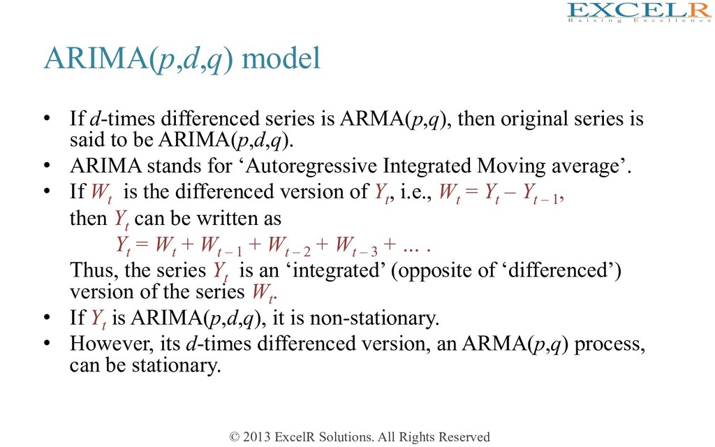
107. © 2013 ExcelR Solutions. All Rights Reserved ARIMA(p,d,q) model •  If d-times differenced series is ARMA(p,q), then original series is said to be ARIMA(p,d,q). •  ARIMA stands for ‘Autoregressive Integrated Moving average’. •  If Wt is the differenced version of Yt , i.e., Wt = Yt – Yt – 1 , then Yt can be written as Yt = Wt + Wt – 1 + Wt – 2 + Wt – 3 + … . Thus, the series Yt is an ‘integrated’ (opposite of ‘differenced’) version of the series Wt . •  If Yt is ARIMA(p,d,q), it is non-stationary. •  However, its d-times differenced version, an ARMA(p,q) process, can be stationary.
108. © 2013 ExcelR Solutions. All Rights Reserved Box-Jenkins ARIMA model-building •  Model identification –  If the time plot ‘looks’ non-stationary, difference it until the plot looks stationary –  Look at ACF and PACF plots for possible clue on model order (p, q) –  When in doubt (regarding choice of p and q), use the principle of parsimony: A simple model is better than a complex model •  Estimate model parameters •  Check residuals for health of model •  Iterate if necessary •  Forecast using the fitted model
109. © 2013 ExcelR Solutions. All Rights Reserved THANK YOU