Main topics covered on this talk:
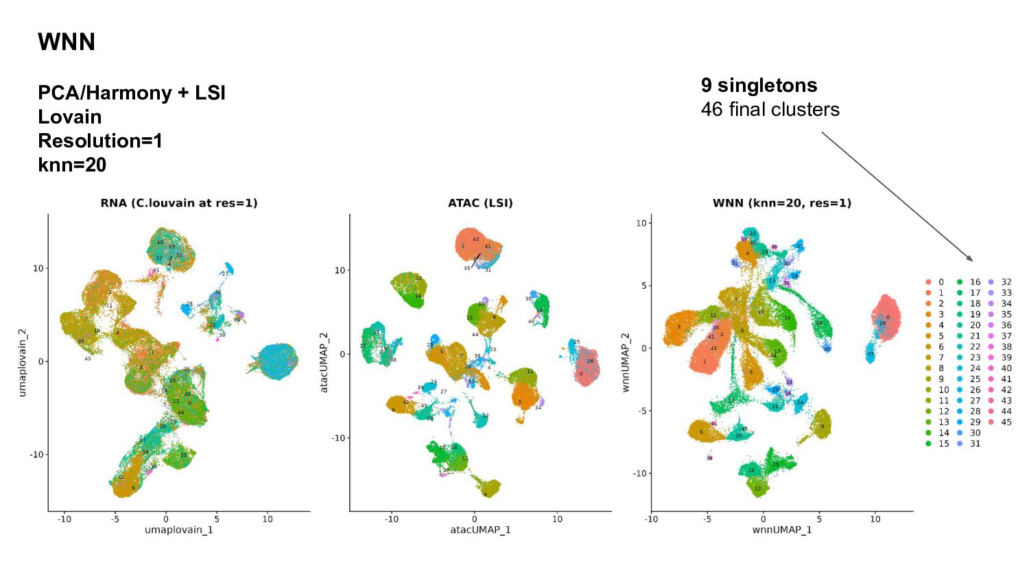
Introducing the Weighted-Nearest Neighbor (WNN) for multimodal analysis
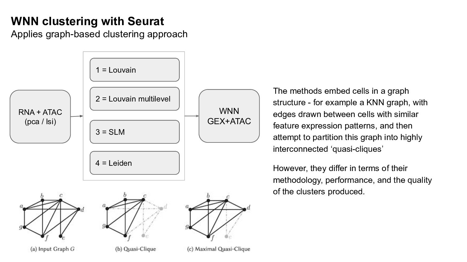
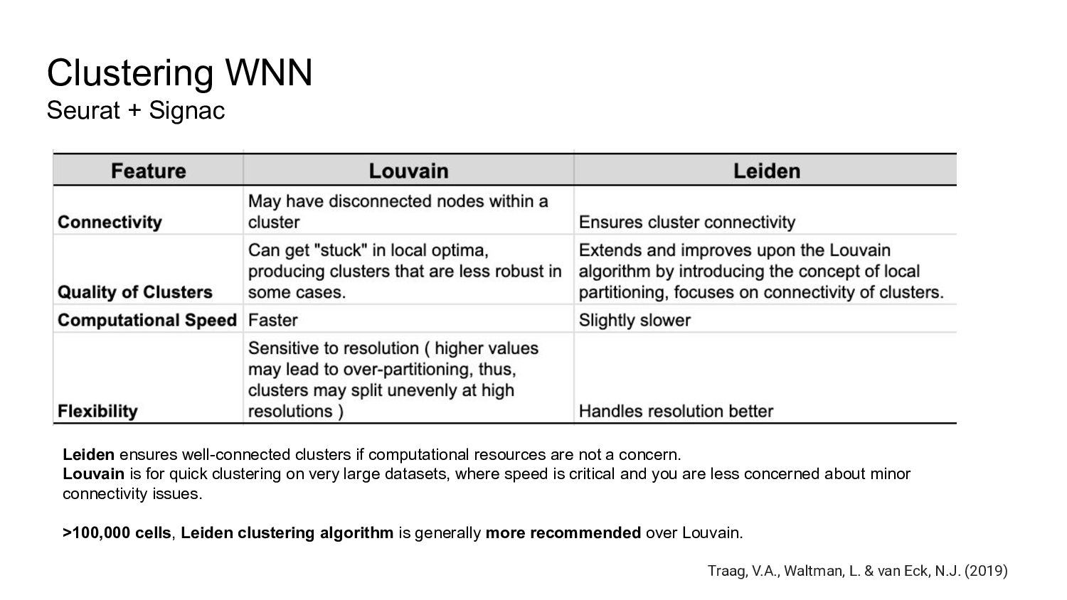
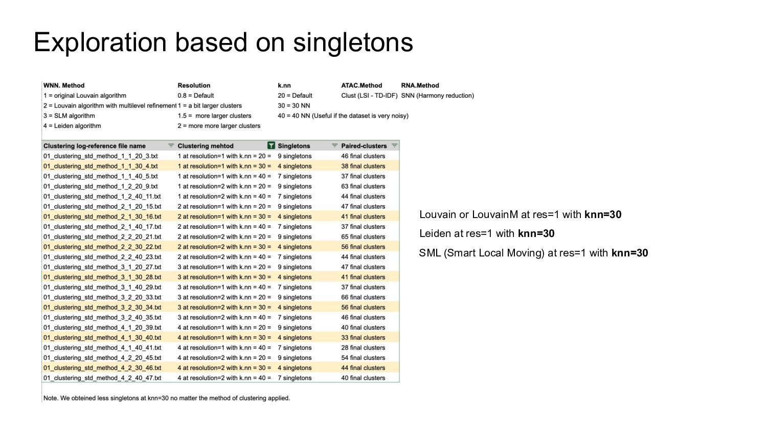
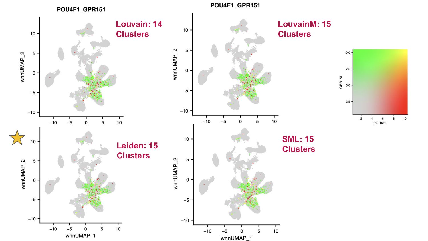
A glance of WNN clustering algorithms available in Seurat
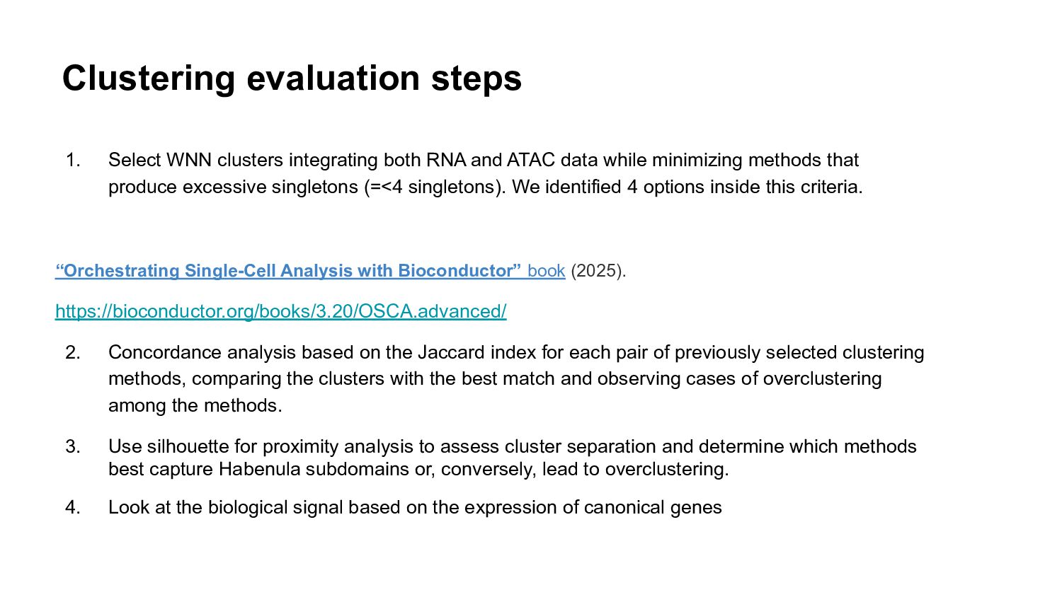
Some clustering evaluation methods:
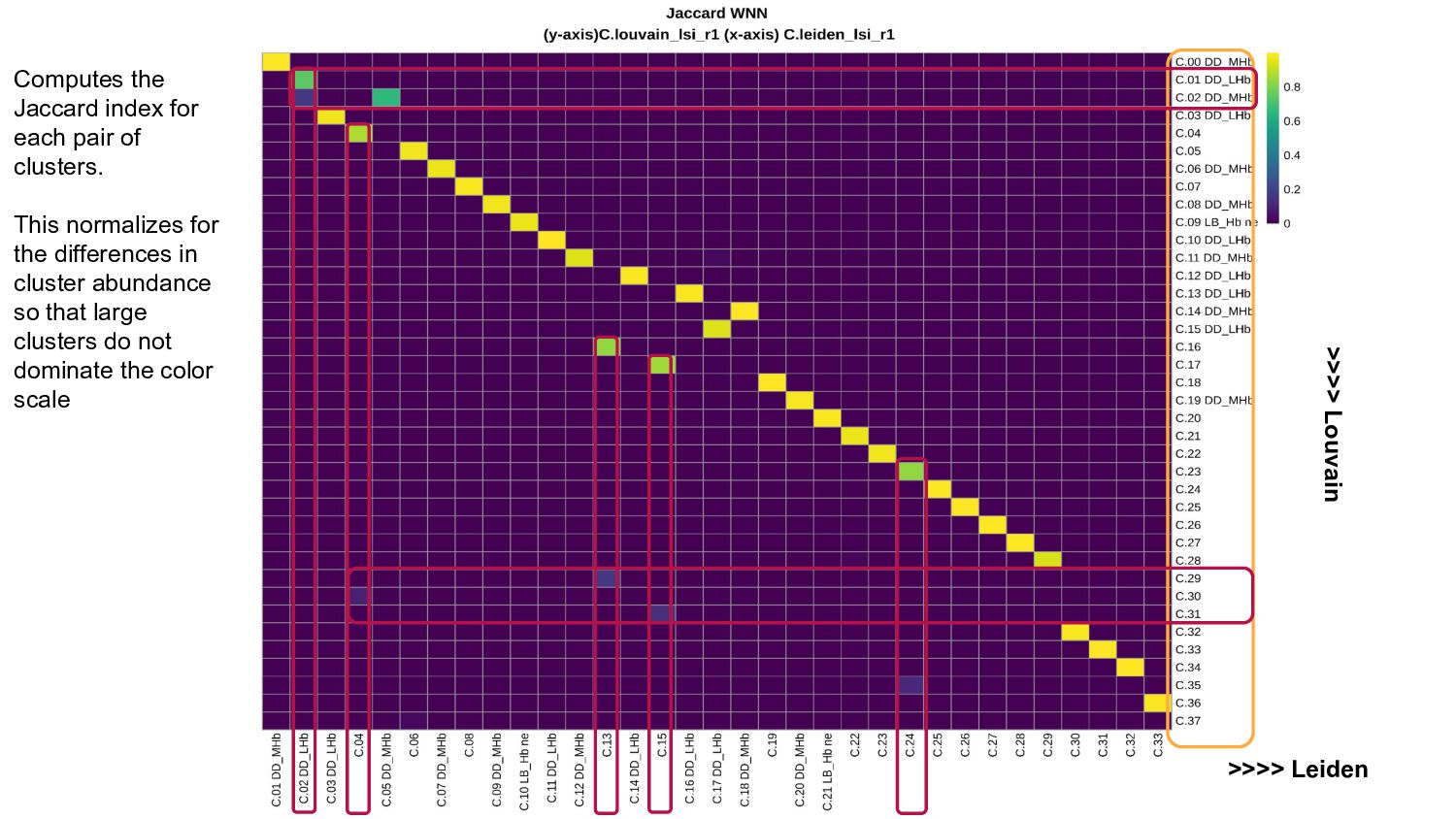
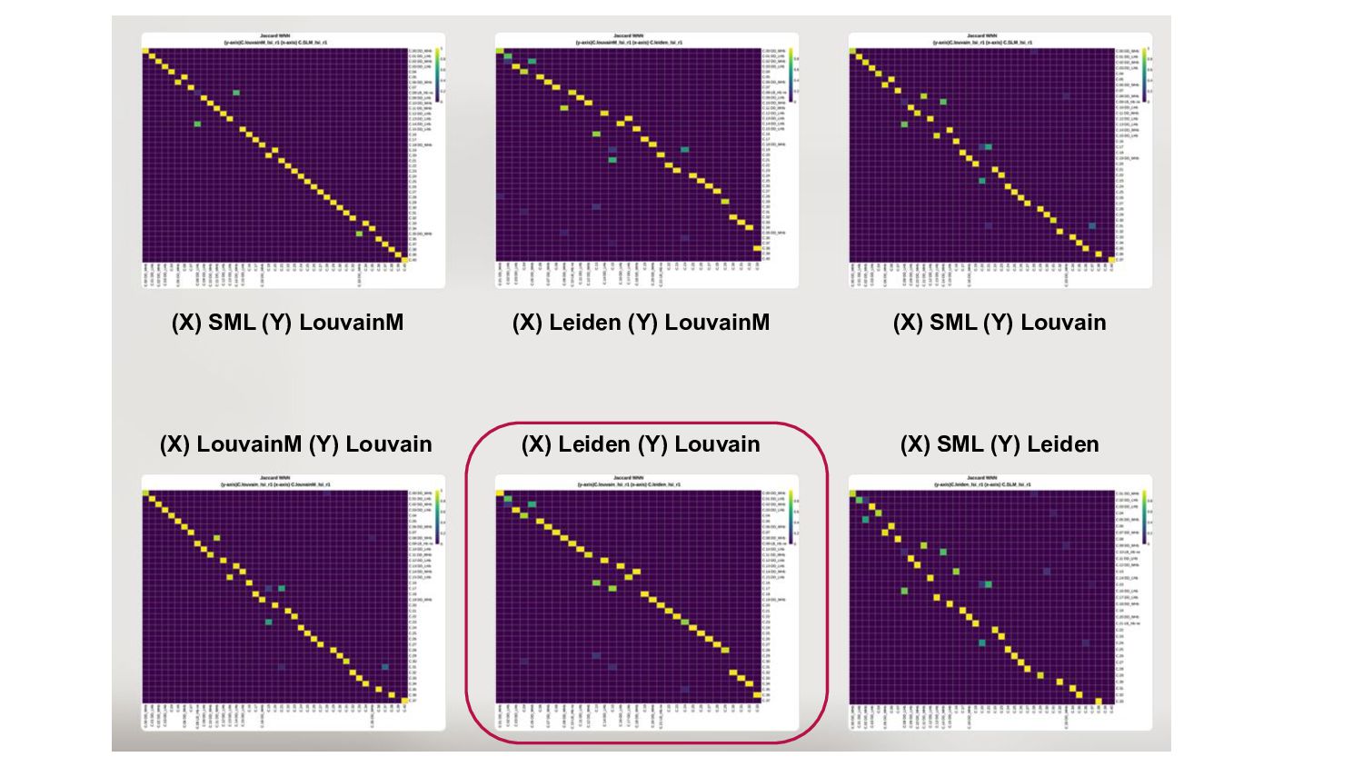
- Concordance analysis based on the Jaccard index
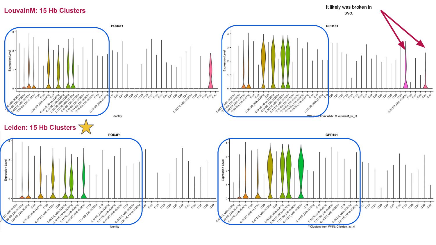
- Looking the biological signal based on the expression of canonical genes
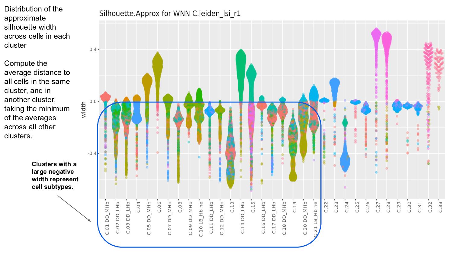
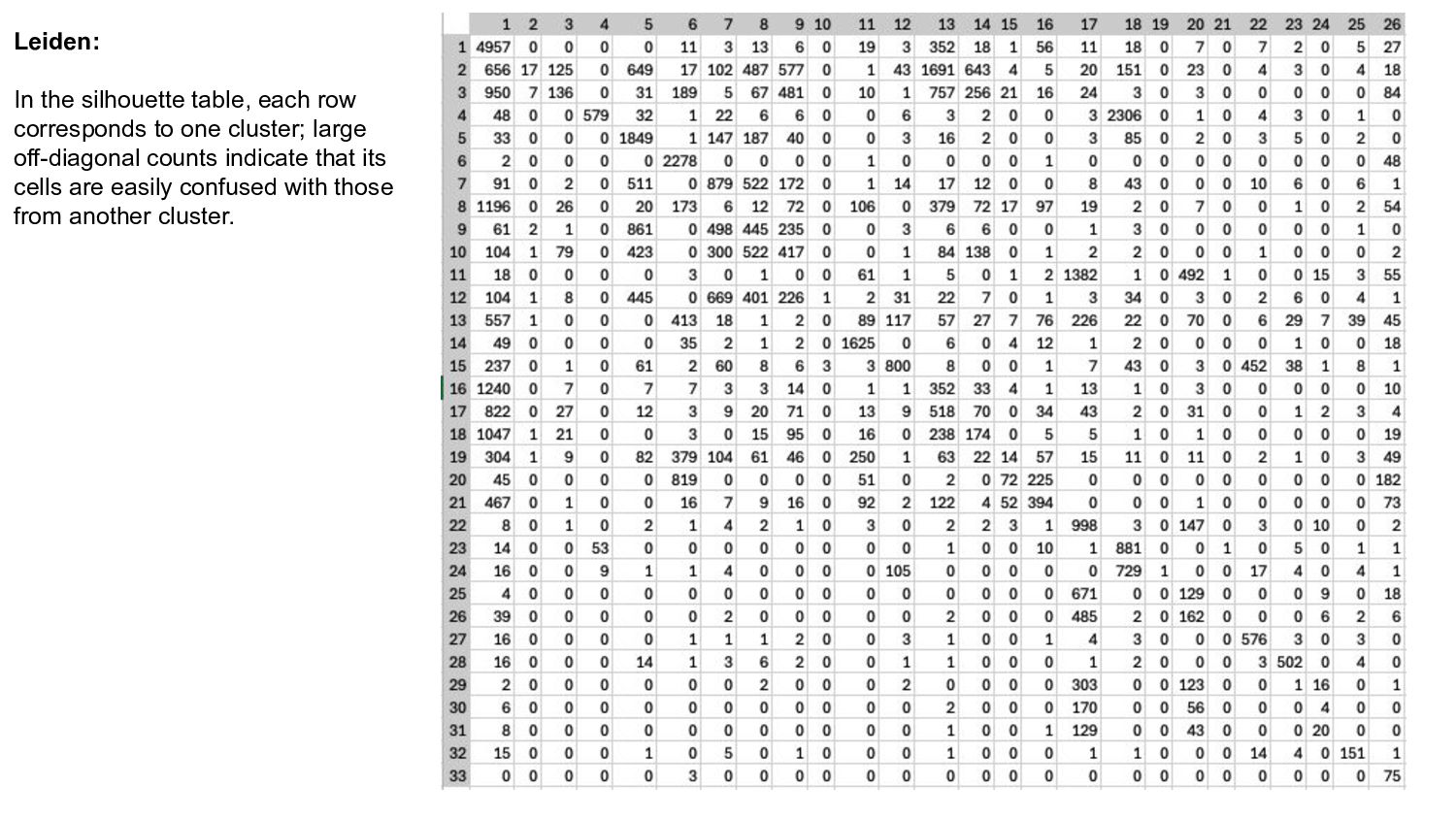
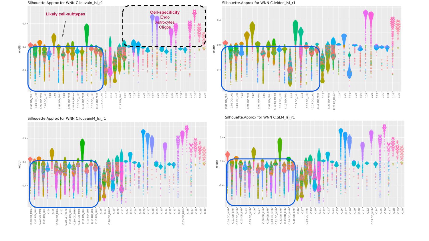
- Proximity Analysis with Silhouette width to assess cluster separation
![LouvainM 15 Clusters % [8.97-0.34] Leiden 15 Clusters % [9.9-2.25]](https://files.speakerdeck.com/presentations/81bf92ee69d94b2db3c82a763802be11/slide_19.jpg)