Monte Carlo Methods

An introduction to the use of random numbers in computational problems and simulations. Code at https://github.com/DanielBrookRoberge/MonteCarloExamples

Transcript

1. Monte Carlo Methods Daniel Brook-Roberge April 19, 2016 Engineering Meeting
2. What are Monte Carlo Methods? • Monte Carlo methods are a family of methods for simplifying difficult computation problems by drawing random numbers. • These numbers are drawn from known probability distributions and are used both directly in formulas and to make decisions.
3. Two Uses For Random Numbers • Mathematical Operations – Random numbers can be drawn as input to some calculation – Often, the inputs to the calculation will obey some probability distribution. • Making Decisions – We can make decisions by drawing a random number between 0 and 1 and comparing it to a probability of a given outcome.
4. All of the examples presented in these slides can be found at: https://github.com/DanielBrookRoberge/MonteCarloExamples
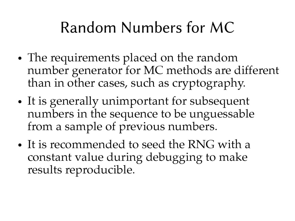
5. Random Numbers for MC • The requirements placed on the random number generator for MC methods are different than in other cases, such as cryptography. • It is generally unimportant for subsequent numbers in the sequence to be unguessable from a sample of previous numbers. • It is recommended to seed the RNG with a constant value during debugging to make results reproducible.
6. Monte Carlo Integration • A simple use of MC methods is for integration of functions. • If we randomly draw points uniformly in a region, we have
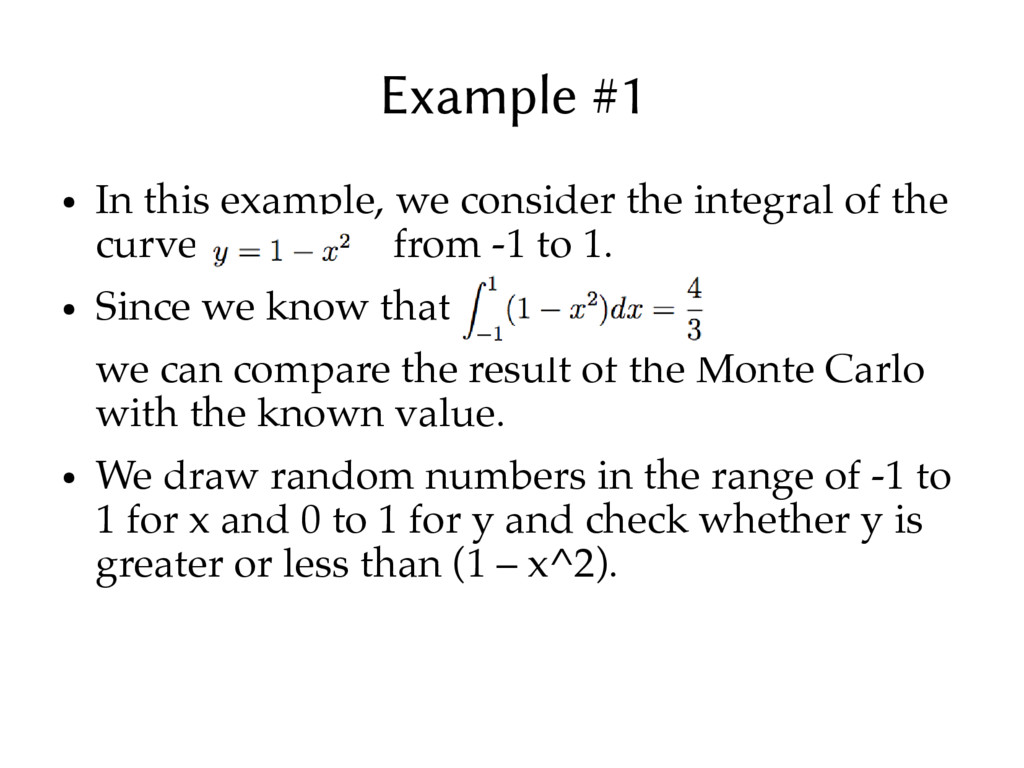
7. Example #1 • In this example, we consider the integral of the curve from -1 to 1. • Since we know that we can compare the result of the Monte Carlo with the known value. • We draw random numbers in the range of -1 to 1 for x and 0 to 1 for y and check whether y is greater or less than (1 – x^2).
8. Accuracy vs Iterations • In general, any Monte Carlo method will be more accurate the more points are drawn. • We can see the value get closer to 4/3 as we draw more points.
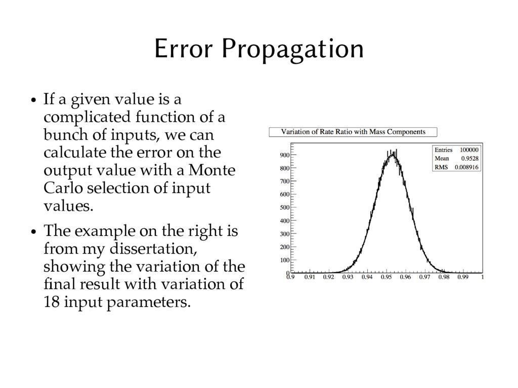
9. Error Propagation • If a given value is a complicated function of a bunch of inputs, we can calculate the error on the output value with a Monte Carlo selection of input values. • The example on the right is from my dissertation, showing the variation of the final result with variation of 18 input parameters.
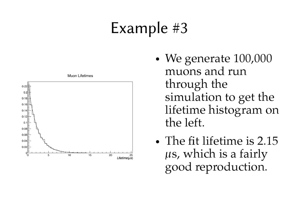
10. Muon Decay • A muon is a type of elementary particle which is unstable. • From the Particle Data Group (pdg.lbl.gov), we see that its mean lifetime is 2.20 µs. • From this, we can derive a probability that the decay occurs in a given time interval, and propagate simulated muons through a series of time steps with Monte Carlo decision making to attempt to reproduce the decay curve.
11. Example #3 • We generate 100,000 muons and run through the simulation to get the lifetime histogram on the left. • The fit lifetime is 2.15 µs, which is a fairly good reproduction.
12. Physics Simulation • The fourth example is a “physics” simulation of a particle beam with simple interactions. • There is an idealized detector which accumulates deposited energy. • The basic method involves randomly selecting initial conditions, then stepping along the particle path making random decisions about the different interaction types. • The annotated source code can be found in the repository.
13. Summary • Monte Carlo methods speed up complicated tasks through the use of randomness. • The main uses for the random numbers are as inputs to calculations or to make decisions. • Randomly sampling high dimension spaces is much faster than a comparable deterministic calculation. • Simulations using Monte Carlo decision making can simulate systems with a wide variety of possible interactions.