Introduction to Gibbs Sampling

Transcript

1. Introduction to Gibbs Sampling David Haber 20.01.2014 David Haber Introduction to Gibbs Sampling
2. Why? Big Question: How do we sample from a probability distribution? Easy: P(X = 0) = 0.5 and P(X = 1) = 0.5 Hard: We want to draw from some joint distribution p(θ1, θ2, ..., θn). The distribution is so complex (no factorization, dependencies, ...) that sampling from it directly is not feasible. Example: p(v, h) = 1 Z exp{−E(v, h)} David Haber Introduction to Gibbs Sampling
3. MCMC - What is a Markov chain? A Markov chain is a stochastic process in which future states are independent of past states given the present state. Consider a draw of θ(t) to be a state at time t. The next draw θ(t+1) is dependent only on the current draw θ(t) and not on any past draws. This satisfies the Markov property: p(θ(t+1)|θ(1), θ(2), ..., θ(t)) = p(θ(t+1)|θ(t)) (1) Example: Google’s Page Rank algorithm David Haber Introduction to Gibbs Sampling
4. MCMC - What is a Markov chain? What are the rules governing how the chain jumps from one state to another at each period? kxk transition matrix P denoted by p(θ(t+1) = x|θ(t) = y). David Haber Introduction to Gibbs Sampling
5. MCMC - What is a Markov chain? The process has k states. 1 Starting distribution (0) (1xk) 2 (1) = (0) ×P 3 (2) = (1) ×P 4 ... 5 (t) = (t−1) ×P = (0) ×Pt David Haber Introduction to Gibbs Sampling
6. MCMC - Stationary Distribution Define a stationary distribution π to be some such that π = πP. We say π is a stationary distribution if it is invariant with respect to the transition matrix. Design Markov chain such that it will converge to π regardless of the starting point and that π is our desired posterior distribution p(θ|y). David Haber Introduction to Gibbs Sampling
7. MCMC - Monte Carlo Simulation If the Markov chain is ergodic it has a unique stationary distribution. A Markov chain is ergodic if for our finite state space Ω and transition matrix P ∃t such that ∀x, y ∈ Ω, Pt xy > 0 (2) David Haber Introduction to Gibbs Sampling
8. MCMC - Monte Carlo Simulation Markov chain Monte Carlo methods produce samples from certain probability distributions by setting up a Markov Chain that converges to its unique stationary distribution distribution. David Haber Introduction to Gibbs Sampling
9. MCMC - Monte Carlo Simulation In Bayesian statistics, there are generally two MCMC algorithms that we use: the Gibbs Sampling and the Metropolis-Hastings algorithm. David Haber Introduction to Gibbs Sampling
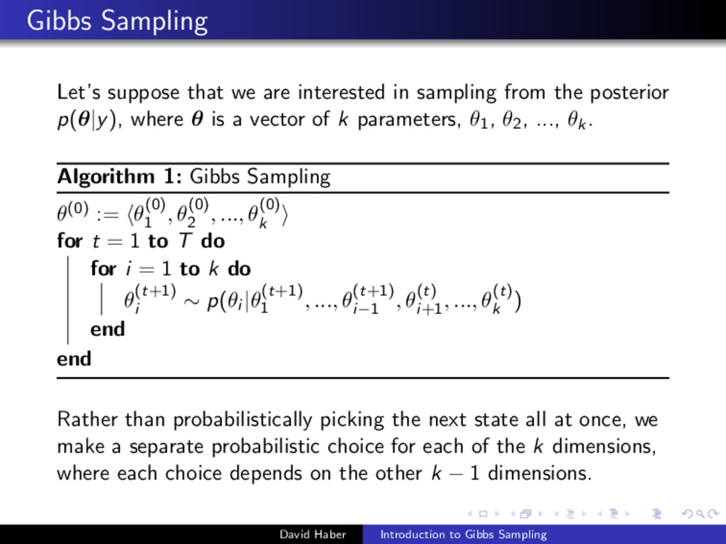
10. Gibbs Sampling Let’s suppose that we are interested in sampling from the posterior p(θ|y), where θ is a vector of k parameters, θ1, θ2, ..., θk. Algorithm 1: Gibbs Sampling θ(0) := θ(0) 1 , θ(0) 2 , ..., θ(0) k for t = 1 to T do for i = 1 to k do θ(t+1) i ∼ p(θi |θ(t+1) 1 , ..., θ(t+1) i−1 , θ(t) i+1 , ..., θ(t) k ) end end Rather than probabilistically picking the next state all at once, we make a separate probabilistic choice for each of the k dimensions, where each choice depends on the other k − 1 dimensions. David Haber Introduction to Gibbs Sampling
11. Back to RBMs RBMs are so called undirected graphical models (or Markov Random fields - MRFs) Figure : The undirected graph of an RBM with 3 hidden and 4 visible variables. David Haber Introduction to Gibbs Sampling
12. Back to RBMs Note: independence between the variables in one layer Gibbs sampling can be performed in two sub steps: sampling a new state h for the hidden neurons based on p(h|v) and sampling a state v for the visible layer based on p(v|h). This is also referred to as block Gibbs sampling. David Haber Introduction to Gibbs Sampling
13. Back to RBMs h(n+1) ∼ sigm(W v(n) + c) (3) v(n+1) ∼ sigm(W h(n+1) + b) (4) As t → ∞, samples (v(t), h(t)) are guaranteed to be accurate samples of p(v, h). David Haber Introduction to Gibbs Sampling
14. Contrastive Divergence (CD-k) Contrastive Divergence uses two tricks to speed up the sampling process: initialize the Markov chain with a training example (close to having converged) do not wait for chain to converge; obtain samples after k-steps of Gibbs sampling (k = 1 works surprisingly well!) David Haber Introduction to Gibbs Sampling
15. Further reading D. Koller and N. Friedman. Probabilistic Graphical Models: Principles and Techniques. MIT Press, 2009. P. Resnik and E. Hardisty. Gibbs Sampling for the Uninitiated. 2010. P. Lam. MCMC Methods: Gibbs Sampling and the Metropolis-Hastings Algorithm. Harvard Lecture Slides. A. Fischer. An Introduction to Restricted Boltzmann Machines, Progress in Pattern Recognition, Image Analysis, Computer Vision, and Applications. Springer Berlin Heidelberg, 2012. 14-36. http://deeplearning.net/tutorial/rbm.html David Haber Introduction to Gibbs Sampling