Computationally Viable Handling of Beliefs in Arguments for Persuasion

Talk @ICTAI16

Transcript

1. Computationally Viable Handling of Beliefs in Arguments for Persuasion Emmanuel Hadoux and Anthony Hunter November 6, 2016 University College London EPSRC grant Framework for Computational Persuasion
2. Introduction
3. Persuasion problems • One agent (the proponent) tries to persuade the other (the opponent) • e.g., doctor persuading a patient to quit smoking, a salesman, a politician, ... 1
4. Persuasion problems • One agent (the proponent) tries to persuade the other (the opponent) • e.g., doctor persuading a patient to quit smoking, a salesman, a politician, ... • the agents exchange arguments during a persuasion dialogue 1
5. Persuasion problems • One agent (the proponent) tries to persuade the other (the opponent) • e.g., doctor persuading a patient to quit smoking, a salesman, a politician, ... • the agents exchange arguments during a persuasion dialogue • These arguments are connected by an attack relation 1
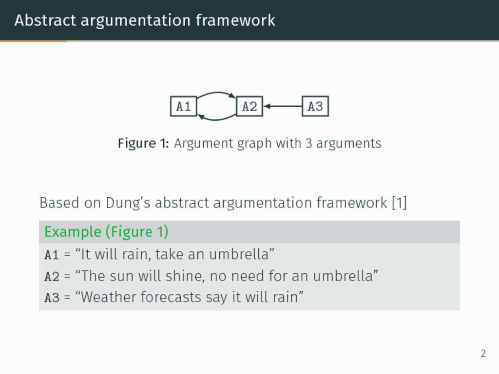
6. Abstract argumentation framework A1 A2 A3 Figure 1: Argument graph with 3 arguments Based on Dung’s abstract argumentation framework [1] Example (Figure 1) A1 = “It will rain, take an umbrella” A2 = “The sun will shine, no need for an umbrella” A3 = “Weather forecasts say it will rain” 2
7. Purpose of the work The objective for the proponent: 1. Have an argument or a set of arguments holding at the end of the dialogue 3
8. Purpose of the work The objective for the proponent: 1. Have an argument or a set of arguments holding at the end of the dialogue 2. Have these arguments believed by the opponent 3
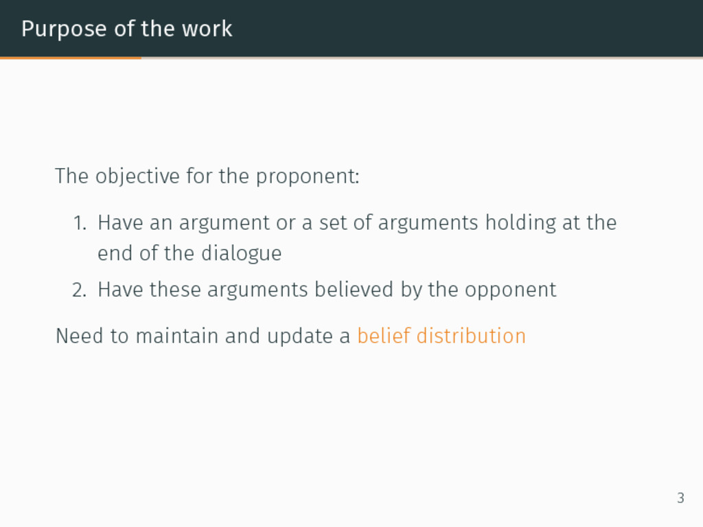
9. Purpose of the work The objective for the proponent: 1. Have an argument or a set of arguments holding at the end of the dialogue 2. Have these arguments believed by the opponent Need to maintain and update a belief distribution 3
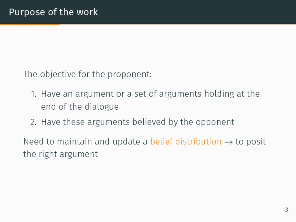
10. Purpose of the work The objective for the proponent: 1. Have an argument or a set of arguments holding at the end of the dialogue 2. Have these arguments believed by the opponent Need to maintain and update a belief distribution → to posit the right argument 3
11. Belief distribution Epistemic approach to probabilistic argumentation (e.g., [2]) Definition Let G = ⟨A, R⟩ be an argument graph. Each X ⊆ A is called a model. A belief distribution P over 2A is such that ∑ X⊆A P(X) = 1 and P(X) ∈ [0, 1], ∀X ⊆ A. The belief in an argument A is P(A) = ∑ X⊆A s.t. A∈X P(X). 4
12. Belief distribution Epistemic approach to probabilistic argumentation (e.g., [2]) Definition Let G = ⟨A, R⟩ be an argument graph. Each X ⊆ A is called a model. A belief distribution P over 2A is such that ∑ X⊆A P(X) = 1 and P(X) ∈ [0, 1], ∀X ⊆ A. The belief in an argument A is P(A) = ∑ X⊆A s.t. A∈X P(X). If P(A) > 0.5, argument A is accepted. 4
13. Belief distribution Epistemic approach to probabilistic argumentation (e.g., [2]) Definition Let G = ⟨A, R⟩ be an argument graph. Each X ⊆ A is called a model. A belief distribution P over 2A is such that ∑ X⊆A P(X) = 1 and P(X) ∈ [0, 1], ∀X ⊆ A. The belief in an argument A is P(A) = ∑ X⊆A s.t. A∈X P(X). If P(A) > 0.5, argument A is accepted. Example (of a belief distribution) Let A = {A, B} where P({A, B}) = 1/6, P({A}) = 2/3, and P({B}) = 1/6 is a belief distribution. Then, P(A) = 5/6 > 0.5 and P(B) = 2/6 < 0.5. 4
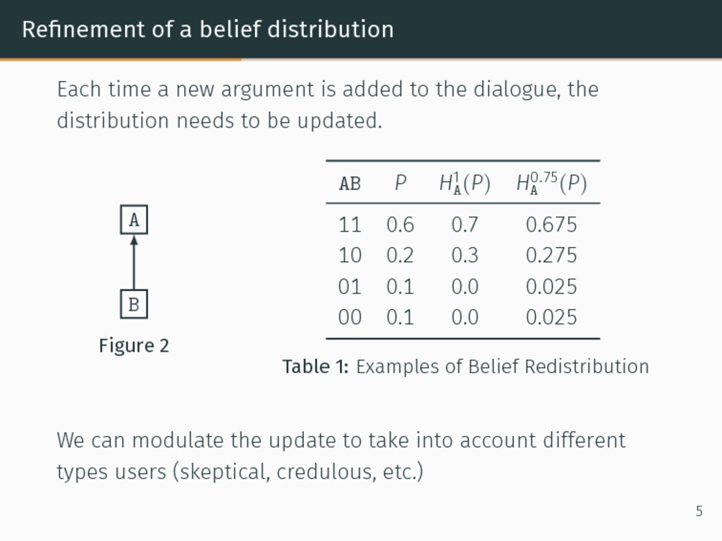
14. Refinement of a belief distribution Each time a new argument is added to the dialogue, the distribution needs to be updated. A B Figure 2 AB P H1 A(P) H0.75 A (P) 11 0.6 0.7 0.675 10 0.2 0.3 0.275 01 0.1 0.0 0.025 00 0.1 0.0 0.025 Table 1: Examples of Belief Redistribution We can modulate the update to take into account different types users (skeptical, credulous, etc.) 5
15. Splitting the distribution
16. Splitting the distribution • 30 arguments → 230 = 1, 073, 741, 824 models → 8.6 gB if treated as a double type 6
17. Splitting the distribution • 30 arguments → 230 = 1, 073, 741, 824 models → 8.6 gB if treated as a double type • Fortunately, they are not all directly linked to each other 6
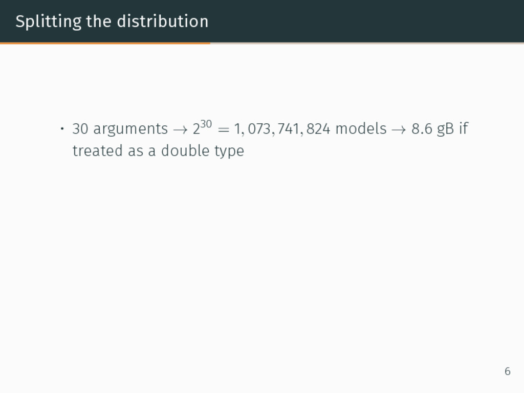
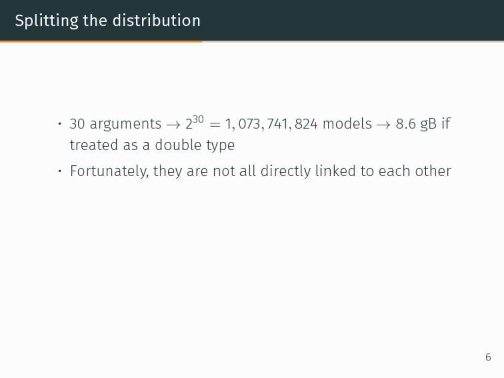
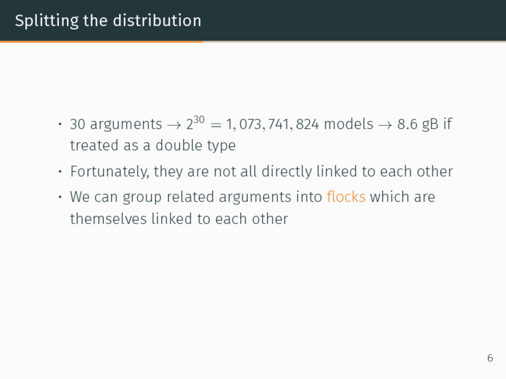
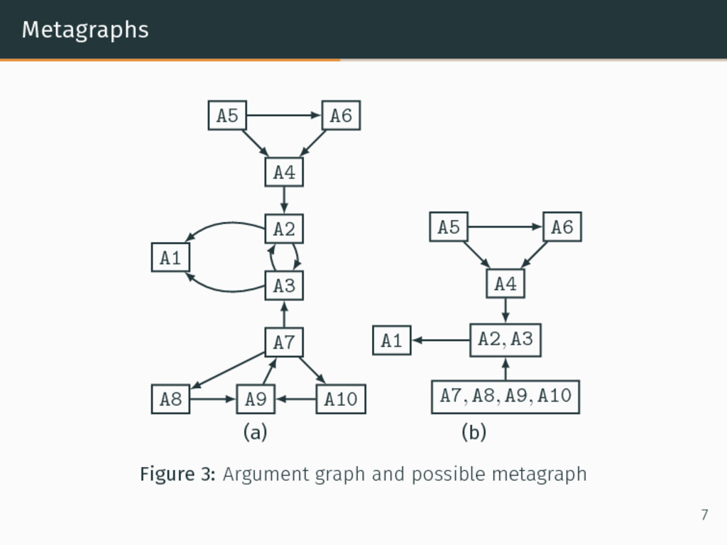
18. Splitting the distribution • 30 arguments → 230 = 1, 073, 741, 824 models → 8.6 gB if treated as a double type • Fortunately, they are not all directly linked to each other • We can group related arguments into flocks which are themselves linked to each other 6
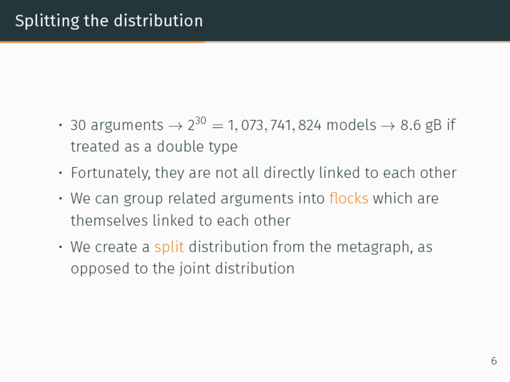
19. Splitting the distribution • 30 arguments → 230 = 1, 073, 741, 824 models → 8.6 gB if treated as a double type • Fortunately, they are not all directly linked to each other • We can group related arguments into flocks which are themselves linked to each other • We create a split distribution from the metagraph, as opposed to the joint distribution 6
20. Metagraphs A1 A2 A3 A4 A5 A6 A7 A8 A9 A10 (a) A1 A2, A3 A4 A5 A6 A7, A8, A9, A10 (b) Figure 3: Argument graph and possible metagraph 7
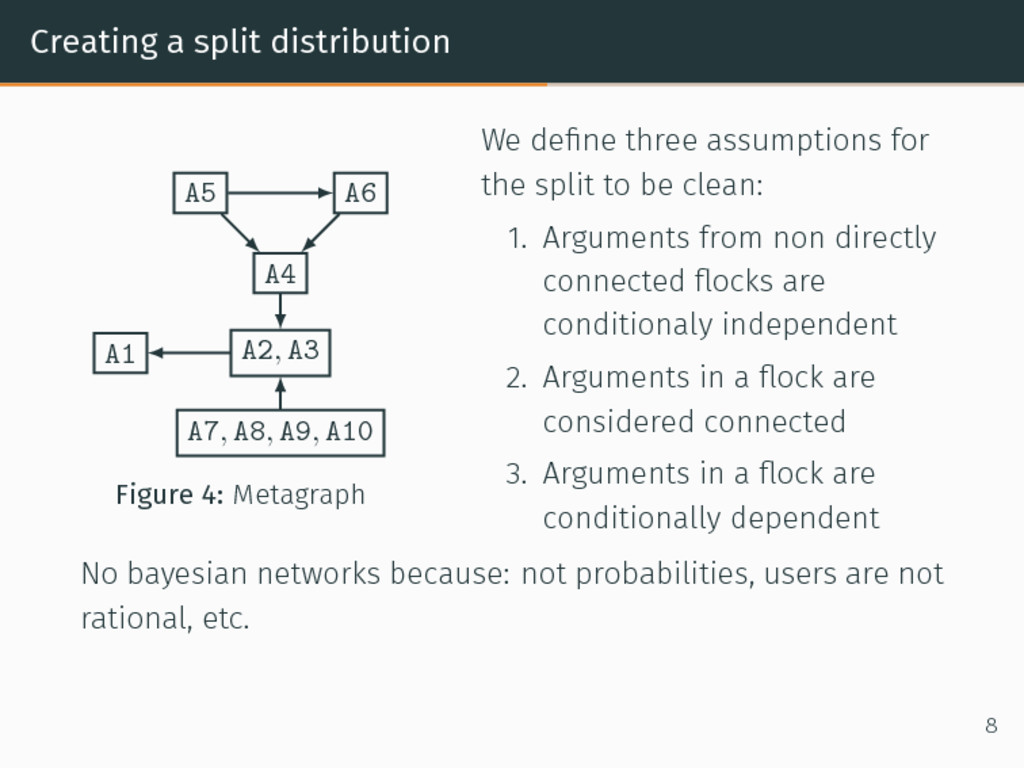
21. Creating a split distribution A1 A2, A3 A4 A5 A6 A7, A8, A9, A10 Figure 4: Metagraph We define three assumptions for the split to be clean: 1. Arguments from non directly connected flocks are conditionaly independent 2. Arguments in a flock are considered connected 3. Arguments in a flock are conditionally dependent No bayesian networks because: not probabilities, users are not rational, etc. 8
22. Creating a split distribution • We can define an optimal, irreducible, split w.r.t. the graph 9
23. Creating a split distribution • We can define an optimal, irreducible, split w.r.t. the graph • However, an irreducible split may not be computable 9
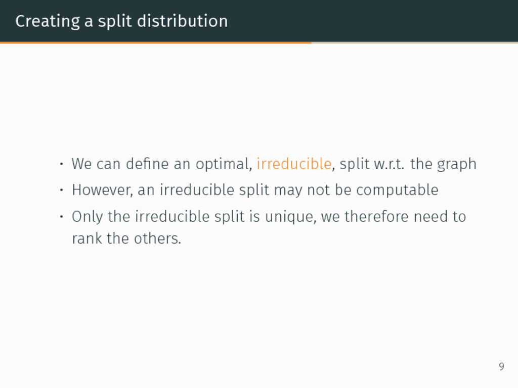
24. Creating a split distribution • We can define an optimal, irreducible, split w.r.t. the graph • However, an irreducible split may not be computable • Only the irreducible split is unique, we therefore need to rank the others. 9
25. Ranking the splits Definition (valuation of a split) x = ∑ A∈A ∑ Pi∈S s.t. A∈E(P) |Pi| and P ≻ P′ iff x < x′. 10
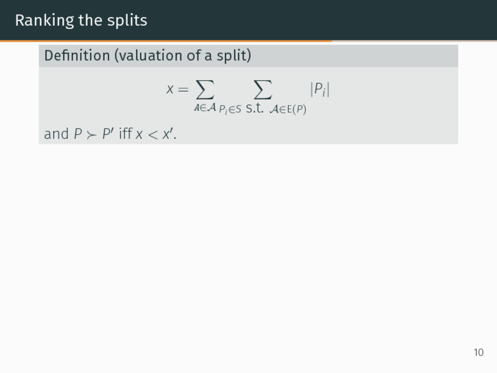
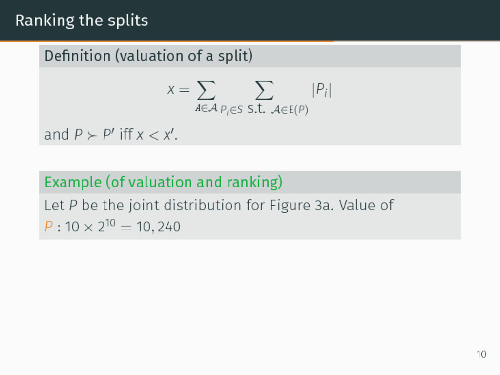
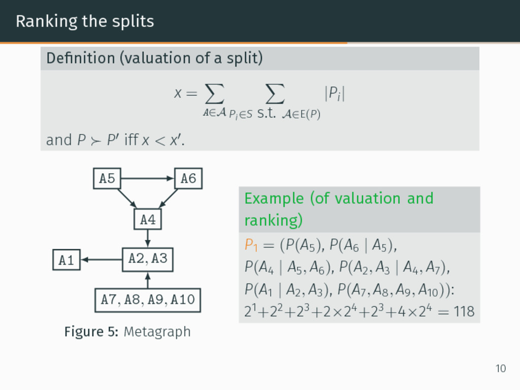
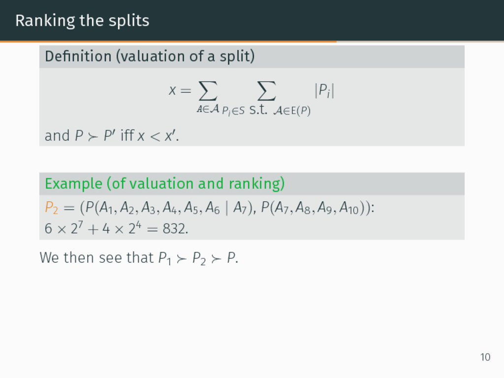
26. Ranking the splits Definition (valuation of a split) x = ∑ A∈A ∑ Pi∈S s.t. A∈E(P) |Pi| and P ≻ P′ iff x < x′. Example (of valuation and ranking) Let P be the joint distribution for Figure 3a. Value of P : 10 × 210 = 10, 240 10
27. Ranking the splits Definition (valuation of a split) x = ∑ A∈A ∑ Pi∈S s.t. A∈E(P) |Pi| and P ≻ P′ iff x < x′. A1 A2, A3 A4 A5 A6 A7, A8, A9, A10 Figure 5: Metagraph Example (of valuation and ranking) P1 = (P(A5), P(A6 | A5), P(A4 | A5, A6), P(A2, A3 | A4, A7), P(A1 | A2, A3), P(A7, A8, A9, A10)): 21+22+23+2×24+23+4×24 = 118 10
28. Ranking the splits Definition (valuation of a split) x = ∑ A∈A ∑ Pi∈S s.t. A∈E(P) |Pi| and P ≻ P′ iff x < x′. Example (of valuation and ranking) P2 = (P(A1, A2, A3, A4, A5, A6 | A7), P(A7, A8, A9, A10)): 6 × 27 + 4 × 24 = 832. We then see that P1 ≻ P2 ≻ P. 10
29. Experiments
30. Splitting the distribution A1 A2, A3 A4 A5 A6 A7, A8, A9, A10 Figure 5: Metagraph • Original graph: 10 arguments → 1,024 values → 8kB • Metagraph: 10 arguments in 6 flocks → 54 values → 432B 11
31. Splitting the distribution A1 A2, A3 A4 A5 A6 A7, A8, A9, A10 Figure 5: Metagraph • Original graph: 10 arguments → 1,024 values → 8kB • Metagraph: 10 arguments in 6 flocks → 54 values → 432B • And the time taken to update. 11
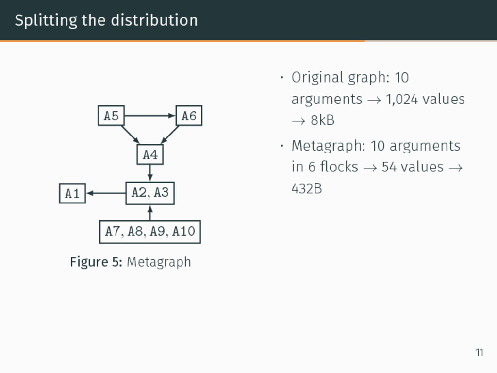
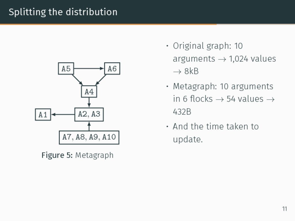
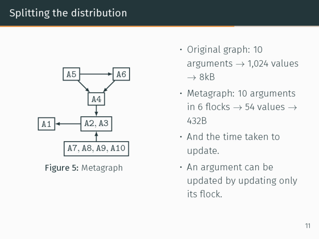
32. Splitting the distribution A1 A2, A3 A4 A5 A6 A7, A8, A9, A10 Figure 5: Metagraph • Original graph: 10 arguments → 1,024 values → 8kB • Metagraph: 10 arguments in 6 flocks → 54 values → 432B • And the time taken to update. • An argument can be updated by updating only its flock. 11
33. Experiments with flocks of different sizes # flocks # links 1 update 50 updates 2 flocks 10 links 2ms 107ms 30 links 6ms 236ms 4 flocks 10 links 1ms 45ms 30 links 3ms 114ms 10 flocks 10 links 0.03ms 1.6ms 30 links 0.06ms 2.5ms Table 2: Computation Time for Updates in Different Graphs of 50 Arguments (in ms) 12
34. Experiments with different numbers of arguments # args Time for 20 updates Comparative % 25 497ns +0% 50 517ns +4% 75 519ns +4% 100 533ns +7% Table 3: Computation Time for 20 Updates (in ns) 13
35. Experiments A new version of the library is currently begin developped in C++ and is available at: https: //github.com/ComputationalPersuasion/splittercell. As a rule of thumb, we should keep flocks to less than 25 arguments each. 14
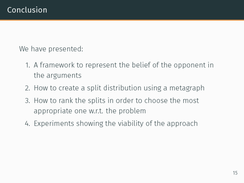
36. Conclusion We have presented: 1. A framework to represent the belief of the opponent in the arguments 2. How to create a split distribution using a metagraph 3. How to rank the splits in order to choose the most appropriate one w.r.t. the problem 4. Experiments showing the viability of the approach 15
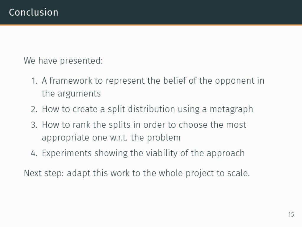
37. Conclusion We have presented: 1. A framework to represent the belief of the opponent in the arguments 2. How to create a split distribution using a metagraph 3. How to rank the splits in order to choose the most appropriate one w.r.t. the problem 4. Experiments showing the viability of the approach Next step: adapt this work to the whole project to scale. 15
38. Thank you! 15
39. Phan Minh Dung. On the acceptability of arguments and its fundamental role in nonmonotonic reasoning, logic programming, and n-person games. Artificial Intelligence, 77:321–357, 1995. Anthony Hunter. A probabilistic approach to modelling uncertain logical arguments. International Journal of Approximate Reasoning, 54(1):47–81, 2013. 15